JAN 20, 2026|11 min read

In our previous architectural overview blog post, we examined the architecture of Snowflake ML's model serving and the process by which a logged model is transformed into a scalable inference service. This post explains the performance optimizations that make our system fast. It details our inference server's development, showing how optimal configuration, no-wait dynamic batching and request pipelining can maximize throughput and maintain low latency with available resources.
To appropriately gauge the advancements made, it is essential to establish a consistent experimental framework and iterate upon it. For our assessment, we incorporated various model types, ranging from decision trees (such as XGBoost) and embedding models (such as Sentence Transformer) to large language models (such as Gemma, chosen to minimize evaluation costs). Nevertheless, for the sake of conciseness and to provide an illustrative overview of our process, this post focuses on a single representative model.
To elaborate all the optimizations we have done, we picked a widely used embedding model, sentence-transformers/all-MiniLM-L6-v2, as an example that leverages GPUs running on a GPU_NV_M compute pool. In this compute pool each node has four A10G GPUs. These are relatively small GPUs but should be sufficient to explain all the optimization techniques. While these optimizations are not model specific, the Sentence Transformer is an excellent representative model for studying GPU behavior.
We set the num_workers to be 8, which means that the four GPUs are split among these eight workers. This also means that the model is copied twice on each GPU, once per worker. For every request, we send only a single row for inference to simulate a real-time interactive inference use case.
We measured end-to-end latency observed from the client, which is outside of the Snowflake network perimeter. This means that the latency number reported in the example in this blog post not only is the inference time but also includes the round trip from client to server. We deployed clients in the same region of the Snowflake account but outside of Snowflake network perimeter to test end-to-end latency, including Snowflake’s network layer.
Also note that we ignored the first few requests in order to account for the cold start issue.
We optimized our inference stack's performance through various experiments, the results of which informed our decisions. The baseline stack, detailed in our architectural overview blog post, consists of a controller and an engine.
As noted, "8" signifies eight engine workers. Our system's baseline is simple: An incoming inference request is immediately assigned to an idle engine worker by the controller. If all workers are busy, the request waits at the proxy. We will now examine the resulting P99 latencies.
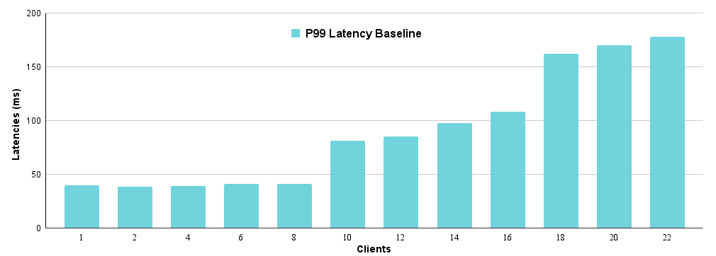
The P99 latency remains around 40 ms for up to eight requests. However, adding a 10th parallel client causes a significant ~40 ms increase in P99 latency. This bump occurs because when the ninth request arrives, all eight inference workers are busy, forcing the ninth request to wait for a worker to become available.
Our initial inference service, using a simple Gunicorn web server with basic worker management, quickly became unscalable due to the mismatch in resource needs between serving and model inference.
GPU vs. CPU work separation: CPU/memory-bound serving operations (request handling, serialization, deserialization, batching) contrast with GPU-bound model inference, especially with accelerators. Combining these distinct components on a single unit caused significant performance degradation and complicated optimal resource allocation.
Efficient thread management: Serialization, deserialization and batching are highly CPU-intensive but parallelizable tasks. Implementing these operations natively via a controller was critical for performance, allowing only the inference engine and its dependencies to remain in Python (engine). This native controller enabled advanced thread management, background monitoring and automated logging without increasing latency.
Processing model inference requests one by one severely underutilizes powerful parallel GPUs, leading to wasted cycles and queuing. Batching multiple requests allows the GPU to process many inputs in nearly the same time as one, dramatically improving utilization and speeding up batched requests.
Traditional dynamic batching systems wait for one of two conditions to be met before processing a batch:
A short timer of just a few milliseconds: This allows inference requests that arrive before this timer runs out to accumulate.
A reached max_batch_size: This is an internal knob that is not exposed to users.
While this system improves GPU utilization and latency under high load, low-QPS scenarios introduce undesirable latency as requests wait for the timer, leading to increased latency, especially with nonuniform incoming requests when the batching condition isn't met.
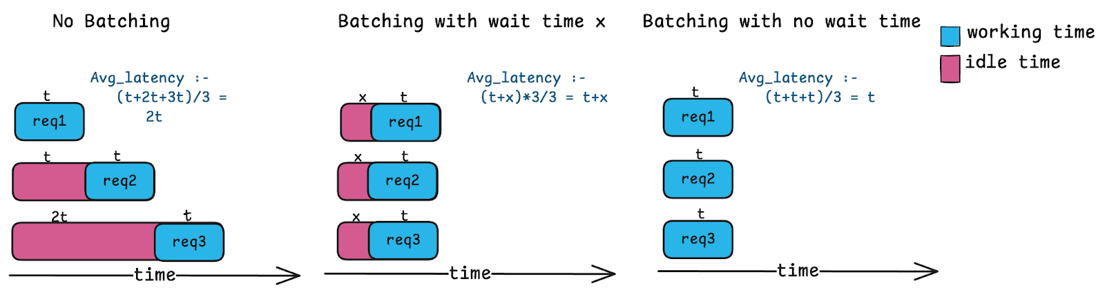
Our approach is different: We batch whatever requests have already arrived at the moment we're ready to process:
Light load: One request waiting? Process it immediately with no delay.
Heavy load: Ten requests waiting? Batch them all and leverage the GPU's parallel power.
This no-wait approach adapts automatically to your traffic patterns. Under light load, you get minimal latency. Under heavy load, you get maximum GPU utilization and reduced queuing, with no tuning required.
To prevent out-of-memory errors caused by batches exceeding available GPU memory, we set a max_batch_size. Requests won't accumulate to a batch beyond this limit, which is automatically tuned for optimal utilization and latency. For the experiments in this example, we set this value to 8.
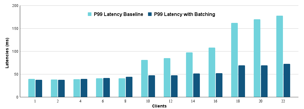
The results clearly show that the large latency spikes from the baseline are eliminated with batching, and the effect is more pronounced with more clients. With 22 clients, batching reduced the p99 latency from 178 ms in the baseline to 73 ms.
In high-parallel inference, the engine worker often waits idly after completing a prediction while the controller prepares the next batch. This pattern of wasted compute capacity also slightly increases inference latencies.
To eliminate idle time, the controller ensures a request is always buffered at the inference worker. This way, the worker immediately processes the next request upon finishing the current one, avoiding the wait for the controller to push a new batch.
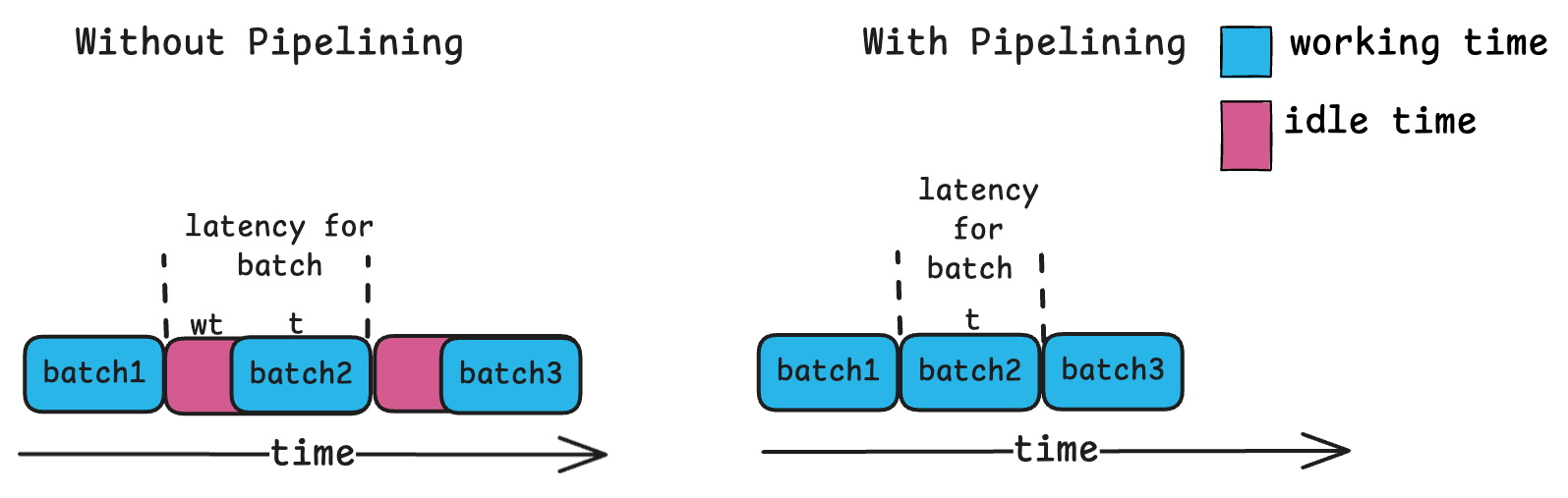
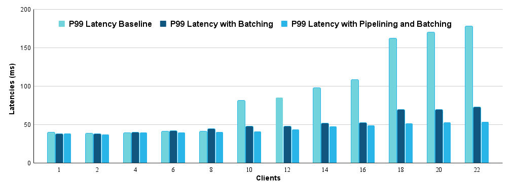
As you can see with a higher number of clients, pipelining gives a good improvement over batching. In the case with 22 clients we saw a p99 latency of 73 ms compared to the 54 ms we achieved with just batching.
To fully illustrate the performance gains, we initially used low concurrency. However, an ideal inference server should maximize resource utilization and gracefully handle traffic spikes. To evaluate this, we stress-tested our system on a single GPU_NV_M node.
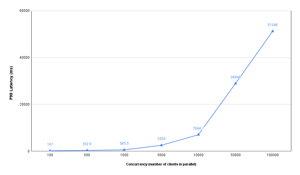
In this example, our dynamic batching architecture's stress test confirms a predictable load-latency relationship. With 1,000 concurrent requests per pod, the system maintained high responsiveness with subsecond P99 latency (~585 ms), preserving resources for traffic spikes. This expected behavior means increased administrative overhead from larger batches accompanies higher load. The system is functioning as designed, optimizing for speed during normal traffic while utilizing full hardware capacity under extreme load.
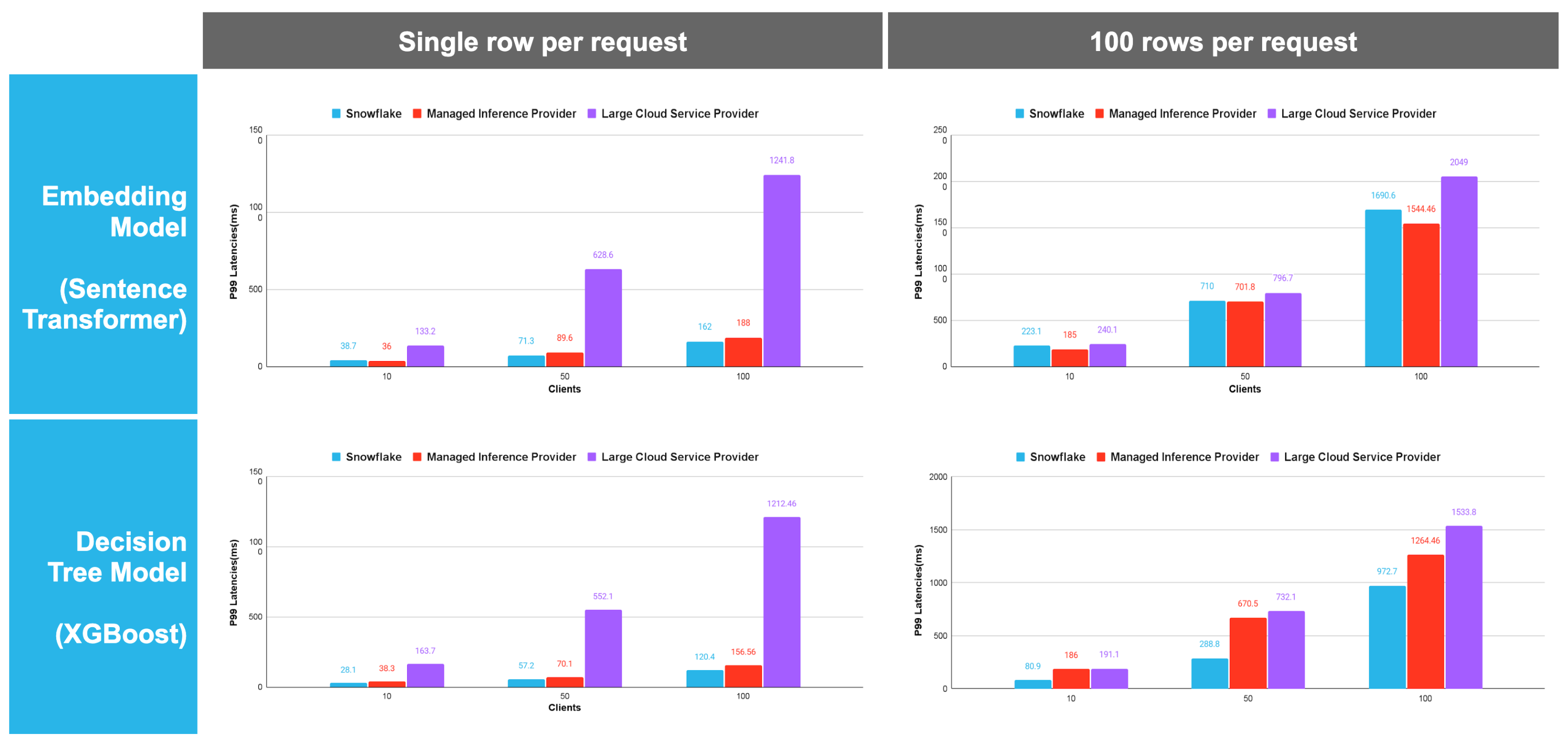
For production-grade decision tree models such as XGBoost, Snowflake delivers up to 10x faster inference latency than legacy cloud providers. In high-concurrency environments (100+ clients), Snowflake’s optimized engine maintains sub-200 ms response times where competitors see much higher performance degradation (compared using equivalent hardware), ensuring a more predictable and cost-effective inference solution for production ML.
Key takeaways:
Significant latency edge at scale: Snowflake consistently maintained lower P99 latencies across both embedding and decision tree models. This advantage becomes most pronounced at 100 concurrent clients, where Snowflake's latency is often a fraction of the "Large Cloud Service Provider" (for example, ~120 ms vs. ~1,212 ms for XGBoost).
Superior batch efficiency: When moving from 1 to 100 rows per request, Snowflake showed better vertical scaling. For the embedding model at 100 clients, Snowflake achieved ~1690 ms while the competition climbed to ~2,049 ms, suggesting a more optimized internal batching engine.
Performance stability: Snowflake’s latency curve was flatter. While competing "serverless" solutions see exponential latency spikes as concurrency (clients) increases, Snowflake’s optimized engine handles high-concurrency workloads with much higher predictability.
Snowflake ML's model serving achieves powerful performance through no-wait dynamic batching and request pipelining. Dynamic batching boosts throughput and lowers perceived latency under heavy load by processing multiple requests simultaneously, eliminating sequential queuing. Request pipelining enables continuous work by pre-queuing the next task, translating small constant-time savings into significant gains at scale. Benchmarks confirm that these optimizations deliver a fast, efficient and scalable experience for demanding ML workloads. Try Snowflake model serving today; the code for the benchmarks is available here.