Why Do We Need Semantic Views? Avoiding Subtle Mistakes in Complex Calculations

In business intelligence (BI), it is very common for vendors such as Snowflake, Tableau, PowerBI and Looker to have a concept of semantic models. They contain the fields that people want to use in order to do an analysis.
If you ask BI folks (like myself) about semantic models, you may get some rambling answers with words such as “grain,” “chasm trap” or “fan trap,” as well as a diatribe about ambiguous join paths and role-playing dimensions. This blog post goes through some of these concepts and provides some context on why these are tricky problems and how semantic views give us the tools to solve them. These tools give us the critical safeguards we need to feel confident about our calculations.
We’ll go through some common analytics pitfalls such as fan and chasm traps and see how they lead to incorrect metrics. We’ll also touch on solutions and discover how addressing the pitfalls with semantic views allows us to focus on the core business questions and not the nuances of query generation.
Joining is hard
This concept is sometimes a little shocking to people. For people who have been joining data for years, it can be hard to understand why it is hard when doing BI or analytics.
The pernicious answer to that is “join explosions.” When you join multiple tables, it is common for one of those tables to have its values duplicated. If you then do aggregations on those values, you get the wrong answer. The problem is that SQL is completely happy with the answer. You asked it to join and then to aggregate the results, and that was valid SQL, but it was not valid analytics, because you double counted values.
Here is an example of this happening, in a pattern called a fan trap:
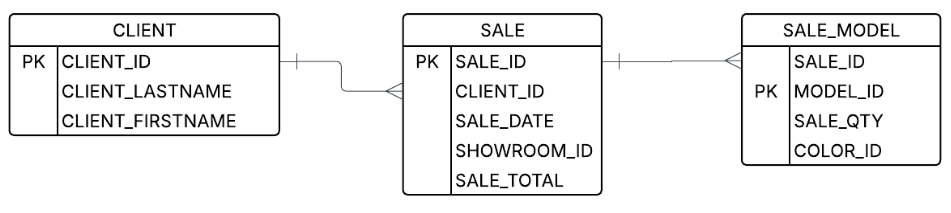
Let’s say a user wants to look at the number of models sold and the total sales price. Well, you know the join keys, and you see the columns — how hard can it be? However, if you do the first join that comes to mind, you will get incorrect results:
-- This will duplicate results and give an incorrect SALE_TOTAL
SELECT CLIENT_LASTNAME, CLIENT_FIRST_NAME, SUM(SALE_QTY), SUM(SALE_TOTAL)
FROM client join sale on (CLIENT_ID = CLIENT_ID)
join SALE_MODEL on (SALE_ID = SALE_ID)
GROUP BY 1, 2
That’s because after you do the joins (but before the aggregation), you start with data that looks something like this:
| SALE_ID | CLIENT_ID | SALE_DATE | SHOWROOM_ID | SALE_TOTAL |
|---|---|---|---|---|
| 1234 | abc123 | 10/10/10 | 4 | 100.00 |
| SALE_ID | MODEL_ID | SALE_QTY | COLOR_ID |
|---|---|---|---|
| 1234 | widget-1 | 2 | yellow |
| 1234 | widget-2 | 1 | red |
| 1234 | widget-2 | 1 | blue |
But after the join, the data has a replicated sale_total field and looks like this:
| CLIENT_LASTNAME | CLIENT_FIRSTNAME | SALE_TOTAL | SALE_QTY | MODEL_ID |
|---|---|---|---|---|
| Waters | Sam | 100.00 | 2 | widget-1 |
| Waters | Sam | 100.00 | 1 | widget-2 |
| Waters | Sam | 100.00 | 1 | widget-2 |
That, unfortunately, gives you incorrect results. The final aggregation will tell you that Sam Waters spent $300 on four items, when in fact he spent $100 on four items. That’s a big difference!
How to do it right
The right way to do a join like this is to do the aggregation before the join. The core principle we need to follow is aggregating the values separately. There are a few ways to do this, but the canonical way is to create subqueries for the different metrics and combine them for the result.
Here is one example of SQL that prevents this case:
WITH sale_agg AS (
-- Aggregate sale totals by client first
SELECT CLIENT_ID,
             SUM(SALE_TOTAL) AS TOTAL_AMOUNT
FROM sale
GROUP BY CLIENT_ID
), model_agg AS (
-- Aggregate quantity by client (joining sale to get the CLIENT_ID)
-- This keeps the qty calculation separate from the sale amount
SELECT s.CLIENT_ID,
            SUM(sm.SALE_QTY) AS TOTAL_QTY
FROM SALE_MODEL sm
     JOIN sale s ON sm.SALE_ID = s.SALE_ID
GROUP BY s.CLIENT_ID
)
SELECT c.CLIENT_LASTNAME,
  c.CLIENT_FIRST_NAME,
  ma.TOTAL_QTY,
  sa.TOTAL_AMOUNT
FROM client c
LEFT JOIN sale_agg sa ON c.CLIENT_ID = sa.CLIENT_ID
LEFT JOIN model_agg ma ON c.CLIENT_ID = ma.CLIENT_ID;
This works because the SALE_MODEL is aggregated before it is joined to SALE, so there is no join explosion. It becomes a one-to-one join.
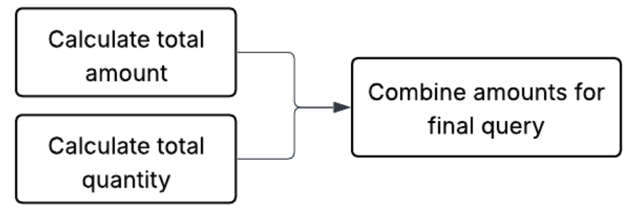
Multistep calculations
You may have noticed above that we needed to break up the query into three different steps. Breaking up calculations into different subqueries is one of the core tricks in de-composing BI queries. In fact, many queries need to get broken up into different steps or different aggregations at different places. These are called multistep calculations.
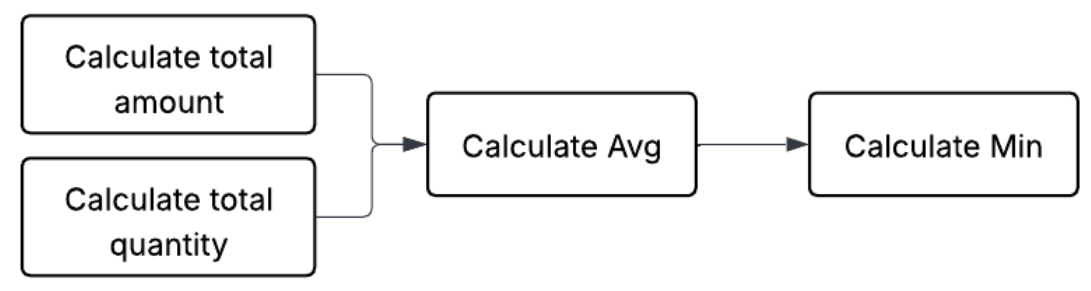
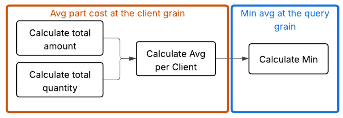
Another example of a multistep calculation would be getting a minimum average model price.
In order to do that, we first need to calculate the totals, which involves taking calculations from each table. Then we need to calculate the average, and finally we need to take the minimum. The key concept here is that we need to describe a sequence of calculations in the right order.
<INCLUDE PREVIOUS EXAMPLE SUB QUERIES>
WITH client_metrics AS (
  -- This is the same logic as the query above
  SELECT c.CLIENT_ID,
         (SUM(sa.TOTAL_AMOUNT) / NULLIF(SUM(ma.TOTAL_QTY), 0)) AS AVG_PRICE
  FROM client c
      JOIN sale_agg sa ON c.CLIENT_ID = sa.CLIENT_ID
      JOIN model_agg ma ON c.CLIENT_ID = ma.CLIENT_ID
  GROUP BY c.CLIENT_ID
)
SELECT MIN(AVG_PRICE) AS HIGHEST_CLIENT_AVG_PRICE
FROM client_metrics;
This is a very simple multistep calculation. However, they can get much more complicated depending on how intricate the question is. In order to reason about such multistep calculations, many semantic models employ the concept of “grain,” or “level of detail.”
Grain, or level of detail
Grain is a way to describe part of a multistep calculation or a calculation that has been run to a particular point. In matching it to SQL, this can be thought of as the “group by” used to aggregate. This has a few interesting properties:
- It is a useful way to mark a spot in a multistep aggregation. Even in complex calculations, it turns out that denoting a level of detail as an aggregation goal is useful.
- At a particular grain, it is guaranteed that the field in the grain will uniquely define a row. This is useful for combining calculations.
Using grain to address the chasm trap
In addition to the fan trap shown above, there is also a chasm trap. In dimensional modeling environments such as snowflake or star schemas, this will often be called a “shared dimension.” This is because it connects two different fact tables that are not naturally connected.
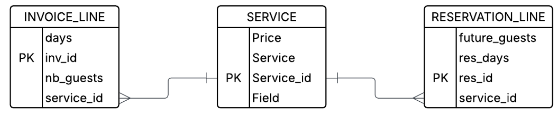
Imagine a case in which a manager wants to issue a query looking at both the NB_GUESTS that have already used a service and the FUTURE_GUESTS that have gotten a reservation. They issue a query with:
-- THE INCORRECT JOIN (The Chasm Trap)
SELECT
    s.SERVICE,
    SUM(il.NB_GUESTS) AS TOTAL_PAST_GUESTS,
    SUM(rl.FUTURE_GUESTS) AS TOTAL_FUTURE_GUESTS
FROM SERVICE s
JOIN INVOICE_LINE il ON s.SERVICE_ID = il.SERVICE_ID
JOIN RESERVATION_LINE rl ON s.SERVICE_ID = rl.SERVICE_ID
WHERE s.SERVICE = 'Guided Tour'
GROUP BY 1;
This straightforward query will unfortunately cause rows to explode. It will create the combinatorics of invoice and reservations for each service_id. To see why this is, imagine that the INVOICE_LINE and RESERVATION_LINE have the following data:
INVOICE_LINE
| INV_ID | SERVICE_ID | NB_GUESTS |
|---|---|---|
| I-99 | S1 | 2 |
| I-100 | S1 | 3 |
RESERVATION_LINE
| RES_ID | SERVICE_ID | FUTURE_GUESTS |
|---|---|---|
| R-501 | S1 | 4 |
| R-502 | S1 | 1 |
The join will then yield the following intermediate table, which duplicated the column.
| SERVICE | INV_ID | NB_GUESTS | RES_ID | FUTURE_GUESTS |
|---|---|---|---|---|
| Guided Tour | I-99 | 2 | R-501 | 4 |
| Guided Tour | I-99 | 2 | R-502 | 1 |
| Guided Tour | I-100 | 3 | R-501 | 4 |
| Guided Tour | I-100 | 3 | R-502 | 1 |
The correct way to handle this is to aggregate both the INVOICE_LINE and the RESERVATION_LINE to the grain of service_id before joining, so that each side has only one row for each service_id.
WITH past_usage AS (
    -- Aggregate guests to the grain of service_id
    SELECT SERVICE_ID, SUM(NB_GUESTS) as TOTAL_PAST
    FROM INVOICE_LINE
    GROUP BY SERVICE_ID
),
future_usage AS (
    -- Aggregate future guests to the grain of service_id
    SELECT SERVICE_ID, SUM(FUTURE_GUESTS) as TOTAL_FUTURE
    FROM RESERVATION_LINE
    GROUP BY SERVICE_ID
)
-- Final Join now has a single row per service_id for each side
SELECT
    s.SERVICE,
    COALESCE(p.TOTAL_PAST, 0) as TOTAL_PAST_GUESTS,
    COALESCE(f.TOTAL_FUTURE, 0) as TOTAL_FUTURE_GUESTS
FROM SERVICE s
LEFT JOIN past_usage p ON s.SERVICE_ID = p.SERVICE_ID
LEFT JOIN future_usage f ON s.SERVICE_ID = f.SERVICE_ID;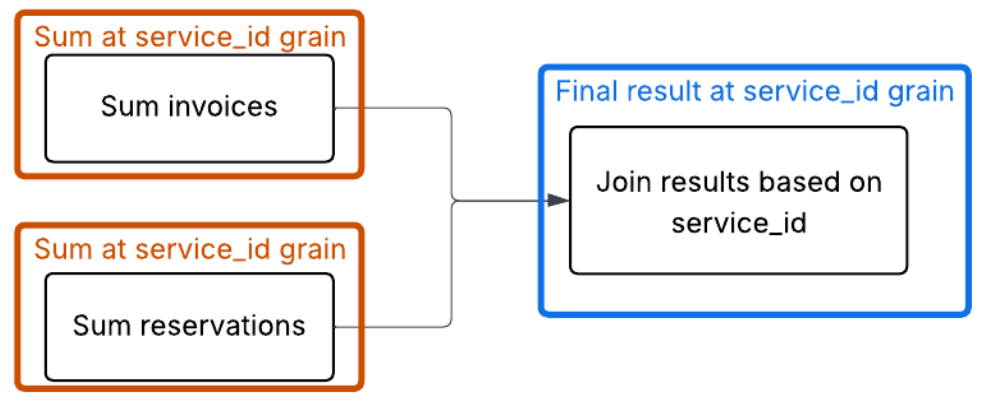
Splitting up aggregations (average of averages is bad)
Now that we have wrapped our head around how aggregations may get split up, let’s look at some mistakes that can happen, even if queries are staged properly. Not all aggregation functions can be broken up so easily.
Average is a good example here. Taking an average of an average tends not to be a good idea. This is because the second average is unweighted, meaning it treats groups of vastly different sizes (such as a service with 100 invoices versus a service with one) as being equally important to the final result.
Look at the following data:
| INV_ID | SERVICE_ID | NB_GUESTS |
|---|---|---|
| I-001 | S1 | 2 |
| I-002 | S1 | 2 |
| I-003 | S1 | 2 |
| I-004 | S1 | 2 |
| I-005 | S1 | 2 |
| I-006 | S1 | 2 |
| I-007 | S1 | 2 |
| I-008 | S1 | 2 |
| I-009 | S1 | 2 |
| I-999 | S2 | 30 |
Step 1A (the incorrect way): Calculate averages per service (the "subaggregations")
- Service S1 average: 18 total guests / 9 invoices = 2.0 guests/inv
- Service S2 average: 30 total guests / 1 invoice = 30.0 guests/inv
Step 1B (the incorrect way): The "average of averages"
(2.0 + 30.0) / 2 = 16.0
The "true average" (the correct way)
To get the true average across all business operations, you must sum all guests and divide by all invoices:
(18 + 30) / (9 + 1) = 48 / 10 = 4.8
A semantic model doesn't just store data; it stores the logic (sum / count). This prevents the “average of averages” error by ensuring that the math is always performed on raw unaggregated rows, even when filtered.
The cost of the "SQL tax"
The examples above — the fan trap, the chasm trap and the fallacy of averages — share a common thread: SQL is a literal language, but business logic is contextual. When we rely on "raw" SQL joins to answer complex questions, we are effectively paying a "SQL tax" every time we build a report. This tax comes in three forms:
- The fragility of manual labor: Writing 50-line CTEs to avoid a fan trap works once. But what happens when a new join is added? Or a filter? The logic is brittle, and the moment it breaks, the data becomes a lie.
- The "CEO question" test: If two different analysts are asked for "average revenue per service" and one uses a flat join while the other uses a CTE, they will provide two different answers. In that moment, the credibility of the entire BI department evaporates.
- Analyst burnout: Your best data minds should be finding insights (for example, "Why is our guided tour revenue dipping?"), not playing "data janitor" by manually auditing joins to make sure a column hasn't exploded by a factor of 10.
Semantic views solve this problem by building analytical safety into the query itself. When you run a query on a semantic view, it will not fall into any of the traps described in this document. Avoiding them is built into the fabric of how they run.
From choosing queries to choosing columns
After you establish a semantic view, your problem becomes simpler. Rather than choosing how to create a query, you choose what dimensions and metrics you want, and the semantic SQL does the rest. Furthermore, you have options. You can either use semantic SQL to have a semantic native interface or use standard SQL and pretend the semantic view is one flat table. You choose the columns; we do the rest.
Here is an example of the fan trap being solved this way. The semantic view locks in how calculations can be done, ensuring that clients (whether human or LLM) will avoid the many possible traps and mistakes.
Create a semantic view using your correct formulations. Create tables to pull in the data you need. Create relationships to define the acceptable join paths. Create dimensions and metrics to expose how to support slicing, dicing and analyzing your data. In particular, metrics can be a critical way to ensure users are calculating important concepts such as revenue in the same, approved way.
CREATE OR REPLACE SEMANTIC VIEW sales_analysis_view
TABLES (
    client AS client
        PRIMARY KEY (client_id),
    sale AS sale
        PRIMARY KEY (sale_id),
    sale_model AS sale_model
        PRIMARY KEY (sale_id, model_id)
)
RELATIONSHIPS (
    sale_to_client AS
        sale (client_id) REFERENCES client,
    sale_model_to_sale AS
        sale_model (sale_id) REFERENCES sale
)
DIMENSIONS (
    client.last_name AS client_lastname,
    client.first_name AS client_first_name
)
METRICS (
    sale.total_amount AS SUM(sale_total),
    sale_model.total_qty AS SUM(sale_qty)
)
COMMENT = 'Semantic view for demonstrating blog post';
The resulting queries are structurally validated. By decoupling the query intent from the join logic, the semantic view ensures the results remain free from traps, regardless of complexity.
Standard SQL uses the semantic view as a table:
SELECT first_name,         last_name,
       AGG(total_amount) AS correct_sale_total,
       AGG(total_qty) AS total_quantity
FROM sales_analysis_view
GROUP BY first_name, last_name;
Semantic SQL directly uses the SEMANTIC_VIEW table function:
SELECT * FROM SEMANTIC_VIEW(
    sales_analysis_view
    METRICS total_amount, total_qty
    DIMENSIONS last_name, first_name
);
From data sprawl to a single source of truth
A semantic view isn't just a technical layer; it’s an insurance policy for your data’s integrity. By defining the "grains" and "relationships" once, the model handles the "agg-before-join" logic automatically.
In a world of data on a Snowflake scale and amazing frontier models, the bottleneck is no longer based on how fast we can query; rather, it's how accurately we can define what we are querying. We don't need more dashboards — we need a unified language that ensures the math is right, no matter who is asking the question.
Snowflake semantic views allow you to build your business and analytics logic into the database to enable safer and smarter analytics. Semantic views are a governed way to define important business metrics. Whether you query them directly from SQL or use an agent to query them, they provide the critical context that is needed by either LLMs or SQL query generation.
Appendix: Can’t LLMs do all of this?
Frontier models are amazing and are getting better at an incredible pace. However, at this point they seem to still be susceptible to the types of problems described above. One of the issues with finding these problems is that they can get very complicated fast.
With a small number of tables, LLMs do a great job. However, I’ve still encountered the traps and averages of averages. Below, I’ve included an example I’ve seen in our evals — see if you can find the error.
It turns out that the same concepts around semantic models that help humans get complicated queries right can also help LLMs.
At Snowflake, we have developed semantic views to codify the core calculations and relationships required for high-precision analytics. Querying these views directly ensures deterministic results, while Snowflake Intelligence and agents use them as a grounded framework to generate more accurate SQL.
LLM generated code with a flaw
The following SQL is an example of a query generated by a very capable LLM over the TPC-DS data set. This query falls into one of the analytical traps mentioned above. Can you tell which one it is? Can you think of the right way to run this query instead?
WITH state_sales_2002 AS (
    SELECT
      ca.ca_state,
      COALESCE(SUM(CASE WHEN d1.d_year = 2002 THEN cs.cs_ext_sales_price END), 0) + COALESCE(SUM(CASE WHEN d2.d_year = 2002 THEN ws.ws_ext_sales_price END), 0) AS total_sales
    FROM AUTOSQL_DATASET_TPCDS.TPCDS.CUSTOMER AS c
    JOIN AUTOSQL_DATASET_TPCDS.TPCDS.CUSTOMER_ADDRESS AS ca
      ON c.c_current_addr_sk = ca.ca_address_sk
    LEFT JOIN AUTOSQL_DATASET_TPCDS.TPCDS.CATALOG_SALES AS cs
      ON c.c_customer_sk = cs.cs_bill_customer_sk
    LEFT JOIN AUTOSQL_DATASET_TPCDS.TPCDS.DATE_DIM AS d1
      ON cs.cs_sold_date_sk = d1.d_date_sk
    LEFT JOIN AUTOSQL_DATASET_TPCDS.TPCDS.WEB_SALES AS ws
      ON c.c_customer_sk = ws.ws_bill_customer_sk
    LEFT JOIN AUTOSQL_DATASET_TPCDS.TPCDS.DATE_DIM AS d2
      ON ws.ws_sold_date_sk = d2.d_date_sk
    GROUP BY
      ca.ca_state
    HAVING
      total_sales > 500000000
), qualifying_states AS (
    SELECT
      ca_state
    FROM state_sales_2002
)
SELECT
  ca.ca_state AS state,
  COUNT(DISTINCT c.c_customer_sk) AS customer_count
FROM AUTOSQL_DATASET_TPCDS.TPCDS.CUSTOMER AS c
JOIN AUTOSQL_DATASET_TPCDS.TPCDS.CUSTOMER_ADDRESS AS ca
  ON c.c_current_addr_sk = ca.ca_address_sk
WHERE
  ca.ca_state IN (
      SELECT
        ca_state
      FROM qualifying_states
  )
  AND NOT ca.ca_state IS NULL /* Exclude the null/empty state */
GROUP BY
  ca.ca_state
ORDER BY
  customer_count ASC
LIMIT 5000
The issue this query falls into is the fan trap. The first CTE tried starting with the customer table and joining through all of the fact tables and dimensions. The problem is that this can cause a join explosion, which would give the wrong aggregation for total_sales.
Example code
If you want to play around at home, here is a snippet of code that should create minimal tables and data so you can see the fan trap in action and how semantic views solve the problem.
-- 1. Client Table (The "One" side)
CREATE OR REPLACE TABLE client (
    client_id INT PRIMARY KEY,
    client_first_name STRING,
    client_lastname STRING
);

-- 2. Sale Table (The "One" side of the sale_model relationship)
CREATE OR REPLACE TABLE sale (
    sale_id INT PRIMARY KEY,
    client_id INT REFERENCES client(client_id),
    sale_total DECIMAL(10,2) -- This is the metric that gets "trapped"
);

-- 3. Sale Model Table (The "Many" side)
CREATE OR REPLACE TABLE sale_model (
    sale_id INT REFERENCES sale(sale_id),
    model_id INT,
    sale_qty INT,
    PRIMARY KEY (sale_id, model_id)
);

INSERT INTO client (client_id, client_first_name, client_lastname)
VALUES (1, 'John', 'Doe');

-- John Doe has ONE sale worth $100.00
INSERT INTO sale (sale_id, client_id, sale_total)
VALUES (101, 1, 100.00);

-- That ONE sale contains TWO different items (Models)
-- Total quantity = 3 (1 + 2)
INSERT INTO sale_model (sale_id, model_id, sale_qty)
VALUES
    (101, 501, 1), -- Item 1
    (101, 502, 2); -- Item 2


-- Semantic View that models the table hierarchy
CREATE OR REPLACE SEMANTIC VIEW sales_analysis_view
TABLES (
    client AS client
        PRIMARY KEY (client_id),
    sale AS sale
        PRIMARY KEY (sale_id),
    sale_model AS sale_model
        PRIMARY KEY (sale_id, model_id)
)
RELATIONSHIPS (
    sale_to_client AS
        sale (client_id) REFERENCES client,
    sale_model_to_sale AS
        sale_model (sale_id) REFERENCES sale
)
DIMENSIONS (
    client.last_name AS client_lastname,
    client.first_name AS client_first_name
)
METRICS (
    sale.total_amount AS SUM(sale_total),
    sale_model.total_qty AS SUM(sale_qty)
)
COMMENT = 'Semantic view for sales analysis';

-- Correct SQL that queries over the semantic view, sales_analysis_view, as if it were a regular view
SELECT first_name,
       last_name,
       AGG(total_amount) AS correct_sale_total,
       AGG(total_qty) AS total_quantity
FROM sales_analysis_view
GROUP BY first_name, last_name;

-- Correct SQL that queries over the semantic view, sales_analysis_view, using the SEMANTIC_VIEW table function
SELECT * FROM SEMANTIC_VIEW(
    sales_analysis_view
    METRICS total_amount, total_qty
    DIMENSIONS last_name, first_name
);

-- THE FAN TRAP (Incorrect Result)
-- This returns $200.00 for John Doe because of the "Join Explosion"
SELECT
    c.client_first_name,
    c.client_lastname,
    SUM(s.sale_total) as incorrect_total_sum,
    SUM(sm.sale_qty) as total_qty
FROM client c
JOIN sale s ON c.client_id = s.client_id
JOIN sale_model sm ON s.sale_id = sm.sale_id
GROUP BY 1, 2;

-- Using a union to make the results easier to see:)
SELECT 'Correct result using SQL' as label,
       first_name,
       last_name,
       AGG(total_amount) AS sale_total,
       AGG(total_qty) AS total_quantity
FROM sales_analysis_view
GROUP BY first_name, last_name
UNION ALL BY NAME
SELECT 'Correct result using SEMANTIC_VIEW' as label, * FROM SEMANTIC_VIEW(
    sales_analysis_view
    METRICS total_amount AS sale_total, total_qty  AS total_quantity
    DIMENSIONS last_name, first_name
)
UNION ALL BY NAME
SELECT
    'Incorrect result because of fan trap' as label,
    c.client_first_name as first_name,
    c.client_lastname as last_name,
    SUM(s.sale_total) as sale_total,
    SUM(sm.sale_qty) as total_quantity
FROM client c
JOIN sale s ON c.client_id = s.client_id
JOIN sale_model sm ON s.sale_id = sm.sale_id
GROUP BY 1, 2, 3
;
Author
