Healthcare ML: Breast Cancer Classification with XGBoost

Snowflake for Developers GuidesHealthcare ML: Breast Cancer Classification with XGBoost

Healthcare ML: Breast Cancer Classification with XGBoost

Applied Analytics

Dureti Shemsi

Overview

This guide walks you through an end-to-end machine learning workflow for breast cancer diagnosis using the Wisconsin Diagnostic dataset. You'll build a production-ready XGBoost classification model, evaluate it with clinical metrics, and deploy it to the Snowflake Model Registry for governed, scalable inference — all using Snowflake Notebooks in Workspaces, the new Jupyter-compatible notebook experience with managed CPU and GPU compute, file management, and direct access to governed Snowflake data.

Early detection of breast cancer significantly improves patient outcomes. The model analyzes cell nucleus characteristics from fine needle aspirate (FNA) images to predict whether a tumor is malignant (cancerous) or benign (non-cancerous).

Prerequisites

A Snowflake account in an AWS or Azure commercial region
ACCOUNTADMIN access or equivalent privileges to run the setup script for Part 2
Basic knowledge of Python and SQL
Familiarity with machine learning concepts

What You'll Learn

How to perform exploratory data analysis with statistical visualizations
How to apply feature scaling and compare multiple classification algorithms
How to use 5-fold stratified cross-validation for robust model evaluation
How to analyze feature importance with XGBoost
How to log a model to the Snowflake Model Registry with metrics and version metadata
How to run batch inference using a registered model

What You'll Need

A Snowflake account
Basic understanding of Snowpark and Snowflake ML

What You'll Build

A trained XGBoost classifier with high accuracy and strong ROC AUC
A registered model version in Snowflake Model Registry with logged metrics
A reusable inference workflow via Python and SQL

Set Up Part 1 Notebook

Part 1 does not require any setup script. You only need to create a service and upload the notebook. All work runs inside Snowflake Notebooks in Workspaces — a Jupyter-compatible environment with managed compute and direct access to Snowflake data.

Create Service

Open Snowflake and navigate to Projects > Workspaces
Click the Connect button in the top toolbar
Select Create new service

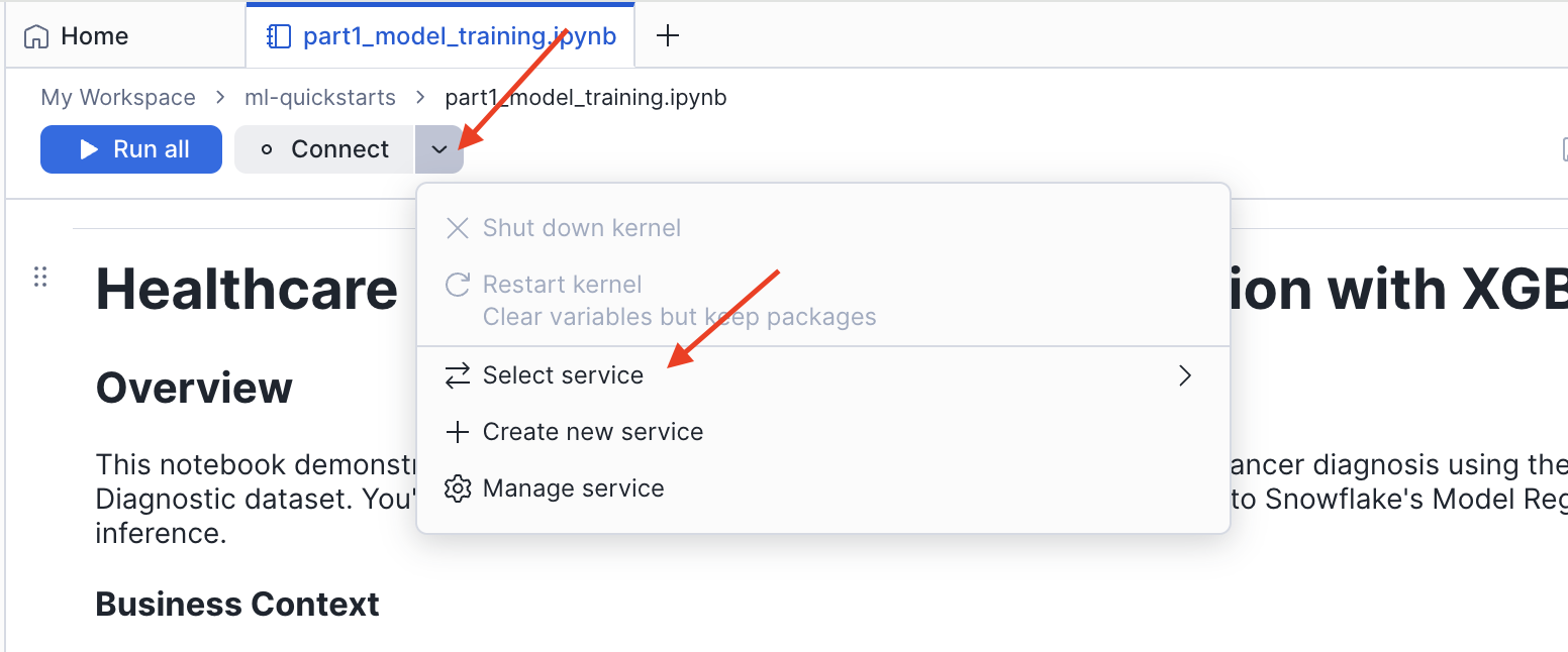
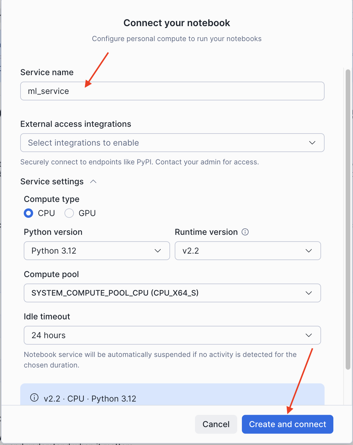
In the Connect your notebook dialog, configure the service:
- Service name: Enter a name (e.g., ml_service)
- External access integrations: Leave empty (not required for Part 1)
- Expand Service settings and set:
  - Compute type: CPU
  - Python version: 3.12
  - Runtime version: v2.2
  - Compute pool: Select an available CPU compute pool
  - Idle timeout: 24 hours (default)
Click Create and connect

Upload Notebook (Part 1)

Download the first notebook to your local machine:

Click this link: 0_start_here.ipynb
On the GitHub page, click the Download raw file button (download icon in the top right)
Save the .ipynb file to your computer

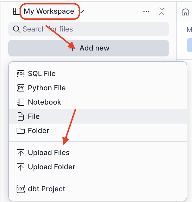
Now upload the notebook into your workspace:

In Projects > Workspaces, click Add new > Upload Files
Select the downloaded 0_start_here.ipynb file
Click on the uploaded file to open it — it is ready to run

NOTE: Part 1 uses Snowflake Notebooks in Workspaces and connects to Snowflake using get_active_session(). Data is loaded from sklearn.datasets — no database or compute pool setup is required.

Load and Explore the Dataset

This section covers loading the Breast Cancer Wisconsin dataset and performing exploratory data analysis to understand class balance and feature distributions.

About the Dataset

The Breast Cancer Wisconsin (Diagnostic) dataset contains 569 samples with 30 features computed from digitized fine needle aspirate (FNA) images of breast masses. Each feature describes characteristics of cell nuclei present in the image.

Feature	Description	Clinical Relevance
Radius	Mean distance from center to perimeter	Larger cells may indicate abnormality
Texture	Standard deviation of gray-scale values	Irregular texture suggests malignancy
Perimeter	Cell boundary length	Related to cell size
Area	Cell size measurement	Malignant cells often larger
Smoothness	Local variation in radius lengths	Irregular shapes are concerning
Compactness	Perimeter² / Area - 1.0	Shape regularity metric
Concavity	Severity of concave portions	Indentations in cell boundary
Concave Points	Number of concave portions	Count of boundary indentations
Symmetry	Symmetry measurement	Asymmetry may indicate problems
Fractal Dimension	"Coastline approximation" - 1	Boundary complexity

For each feature, three statistics are computed — mean, standard error, and worst (mean of 3 largest values) — yielding 30 features total.

Target classes:

0 = Malignant (cancerous) — 212 samples (37.3%)
1 = Benign (non-cancerous) — 357 samples (62.7%)

Load the Data

Run the data loading cell in the notebook:

from sklearn.datasets import load_breast_cancer
import pandas as pd

cancer = load_breast_cancer()
feature_names = [name.replace(' ', '_').upper() for name in cancer.feature_names]
X = pd.DataFrame(cancer.data, columns=feature_names)
y = pd.Series(cancer.target, name="DIAGNOSIS")

Class Distribution Analysis

The dataset has a 1.68:1 Benign:Malignant ratio — a moderate class imbalance. The notebook visualizes this as a bar chart and pie chart. Understanding class balance is critical because:

Imbalanced data can bias models toward the majority class
Accuracy alone becomes misleading with imbalanced classes
Stratified sampling ensures both train and test sets maintain class proportions

Feature Distributions by Diagnosis

The notebook plots histograms of six key mean features (radius, texture, perimeter, area, smoothness, compactness) split by diagnosis class. Features with distinct distributions between classes — such as mean radius and mean area — will be strong predictors.

Correlation Analysis

A correlation heatmap of the 10 mean features reveals that radius, perimeter, and area are highly correlated (geometrically related). This multicollinearity does not harm tree-based models like XGBoost but affects linear model interpretation.

Prepare Data and Compare Models

This section covers train-test splitting, feature scaling, and comparing three classification algorithms using cross-validation.

Train-Test Split

The notebook uses an 80-20 stratified split to maintain class proportions in both sets:

from sklearn.model_selection import train_test_split

X_train, X_test, y_train, y_test = train_test_split(
    X, y, test_size=0.2, random_state=42, stratify=y
)

Split	Size
Training	455 samples (80%)
Test	114 samples (20%)

Feature Scaling

StandardScaler transforms features to have mean=0 and std=1. The scaler is fit only on training data to prevent data leakage:

from sklearn.preprocessing import StandardScaler

scaler = StandardScaler()
X_train_scaled = scaler.fit_transform(X_train)
X_test_scaled = scaler.transform(X_test)

Scaled features are used for Logistic Regression (scale-sensitive). XGBoost is scale-invariant but scaling is applied for a fair comparison.

Model Comparison with 5-Fold Cross-Validation

The notebook compares three algorithms using Stratified K-Fold cross-validation to reduce variance in performance estimates:

Algorithm	Strengths
Logistic Regression	Fast, interpretable, probabilistic
Random Forest	Handles non-linearity, robust to outliers
XGBoost	State-of-the-art accuracy, handles class imbalance

from sklearn.model_selection import StratifiedKFold, cross_val_score

cv = StratifiedKFold(n_splits=5, shuffle=True, random_state=42)

for name, model in models.items():
    scores = cross_val_score(model, X_train, y_train, cv=cv, scoring='accuracy')
    print(f"{name}: {scores.mean():.4f} (+/- {scores.std()*2:.4f})")

XGBoost achieves the highest mean cross-validation accuracy and is selected as the final model.

Evaluate the Model

This section covers evaluating the final XGBoost model on the held-out test set using multiple clinical metrics.

Clinical Metrics for Cancer Screening

Metric	Formula	Clinical Meaning
Accuracy	(TP+TN) / Total	Overall correctness
Precision	TP / (TP+FP)	When predicted malignant, how often correct?
Recall (Sensitivity)	TP / (TP+FN)	Of actual cancers, how many detected?
F1-Score	2 × (P × R) / (P + R)	Harmonic mean of precision/recall
AUC-ROC	Area under ROC curve	Model's discriminative ability

In cancer screening, high recall is critical. A false negative (missed cancer) means the patient goes untreated — potentially fatal. A false positive leads to additional testing, which is manageable.

Confusion Matrix

from sklearn.metrics import confusion_matrix

cm = confusion_matrix(y_test, y_pred)

The confusion matrix shows where the model makes errors. The notebook visualizes this as an annotated heatmap.

ROC Curve

from sklearn.metrics import roc_curve, auc

fpr, tpr, _ = roc_curve(y_test, y_pred_proba)
roc_auc = auc(fpr, tpr)

The XGBoost model achieves a ROC AUC of ~0.99, which falls in the "Excellent" range (0.90–1.00).

Precision-Recall Curve

For imbalanced datasets or when false negatives are costly, PR curves provide more information than ROC alone. The notebook plots the full precision-recall tradeoff at all classification thresholds.

Feature Importance

XGBoost provides feature importance scores based on how frequently each feature is used in tree splits and how much it improves model accuracy:

feature_importance = pd.DataFrame({
    'feature': X.columns,
    'importance': best_model.feature_importances_
}).sort_values('importance', ascending=True).tail(15)

"Worst" features (the largest observed values per nucleus) consistently dominate — extreme cell characteristics are the strongest predictors of malignancy.

Save Artifacts for Part 2

Part 1 ends by saving the trained model and all metrics to /tmp so Part 2 can load them without retraining:

import pickle

artifacts = {
    'best_model': best_model,
    'X_train': X_train,
    'X_test': X_test,
    'y_train': y_train,
    'y_test': y_test,
    'test_accuracy': test_accuracy,
    'test_f1': test_f1,
    'roc_auc': roc_auc,
    'pr_auc': pr_auc,
    'cv_results': cv_results,
    'feature_names': X.columns.tolist()
}

with open('/tmp/breast_cancer_artifacts.pkl', 'wb') as f:
    pickle.dump(artifacts, f)

NOTE: The notebook working directory (/home/udf/) does not persist between sessions. The /tmp path is shared within the same session, which is why Part 2 must be run in the same Snowflake Notebooks session immediately after Part 1.

Deploy to Snowflake Model Registry

Part 2 deploys the trained model to Snowflake Model Registry. This requires running the setup script first to create the necessary database, warehouse, compute pool, and role.

Run the Setup Script

Download the setup.sql script and run it as ACCOUNTADMIN in a new SQL file in Projects > Workspaces, or copy and paste the script below.

Open Snowflake and navigate to Projects > Workspaces
Click Add new > Upload Files to upload the notebook

Copy and paste the following setup script into a new SQL file
Run the entire script as ACCOUNTADMIN

/*
 * ============================================================================
 * Healthcare ML: Breast Cancer Classification with XGBoost
 * ============================================================================
 *
 * Resources created:
 *   - Role: HEALTHCARE_ML_ROLE
 *   - Database: HEALTHCARE_ML
 *   - Schema: HEALTHCARE_ML.DIAGNOSTICS
 *   - Warehouse: HEALTHCARE_ML_WH (for SQL queries and model inference)
 *   - Compute Pool: HEALTHCARE_ML_CPU_POOL (for running the notebook)
 *   - Stage: ARTIFACTS (for persisting data)
 */

USE ROLE ACCOUNTADMIN;

SET USERNAME = (SELECT CURRENT_USER());
SELECT $USERNAME AS CURRENT_USERNAME;

CREATE ROLE IF NOT EXISTS HEALTHCARE_ML_ROLE;
GRANT ROLE HEALTHCARE_ML_ROLE TO USER IDENTIFIER($USERNAME);

CREATE DATABASE IF NOT EXISTS HEALTHCARE_ML;
CREATE SCHEMA IF NOT EXISTS HEALTHCARE_ML.DIAGNOSTICS;

CREATE WAREHOUSE IF NOT EXISTS HEALTHCARE_ML_WH
    WAREHOUSE_SIZE = 'XSMALL'
    AUTO_SUSPEND = 60
    AUTO_RESUME = TRUE;

CREATE COMPUTE POOL IF NOT EXISTS HEALTHCARE_ML_CPU_POOL
    MIN_NODES = 1
    MAX_NODES = 1
    INSTANCE_FAMILY = CPU_X64_XS
    AUTO_SUSPEND_SECS = 300
    AUTO_RESUME = TRUE;

CREATE STAGE IF NOT EXISTS HEALTHCARE_ML.DIAGNOSTICS.ARTIFACTS
    DIRECTORY = (ENABLE = TRUE);

GRANT USAGE ON DATABASE HEALTHCARE_ML TO ROLE HEALTHCARE_ML_ROLE;
GRANT USAGE ON SCHEMA HEALTHCARE_ML.DIAGNOSTICS TO ROLE HEALTHCARE_ML_ROLE;
GRANT CREATE TABLE ON SCHEMA HEALTHCARE_ML.DIAGNOSTICS TO ROLE HEALTHCARE_ML_ROLE;
GRANT CREATE MODEL ON SCHEMA HEALTHCARE_ML.DIAGNOSTICS TO ROLE HEALTHCARE_ML_ROLE;
GRANT CREATE NOTEBOOK ON SCHEMA HEALTHCARE_ML.DIAGNOSTICS TO ROLE HEALTHCARE_ML_ROLE;
GRANT READ, WRITE ON STAGE HEALTHCARE_ML.DIAGNOSTICS.ARTIFACTS TO ROLE HEALTHCARE_ML_ROLE;
GRANT USAGE ON WAREHOUSE HEALTHCARE_ML_WH TO ROLE HEALTHCARE_ML_ROLE;
GRANT USAGE, MONITOR ON COMPUTE POOL HEALTHCARE_ML_CPU_POOL TO ROLE HEALTHCARE_ML_ROLE;
GRANT BIND SERVICE ENDPOINT ON ACCOUNT TO ROLE HEALTHCARE_ML_ROLE;

USE ROLE HEALTHCARE_ML_ROLE;
USE DATABASE HEALTHCARE_ML;
USE SCHEMA DIAGNOSTICS;
USE WAREHOUSE HEALTHCARE_ML_WH;

SELECT '✅ Setup complete! You are ready to run the Healthcare ML notebook.' AS STATUS;

This will create:

A dedicated role: HEALTHCARE_ML_ROLE
A warehouse: HEALTHCARE_ML_WH (XSMALL)
A database: HEALTHCARE_ML
A schema: HEALTHCARE_ML.DIAGNOSTICS
A stage: ARTIFACTS
A compute pool: HEALTHCARE_ML_CPU_POOL (CPU_X64_XS, 1 node)

Upload Notebook (Part 2)

Download the second notebook to your local machine:

Click this link: 1_snowflake_deployment.ipynb
On the GitHub page, click the Download raw file button
Save the .ipynb file to your computer

Upload the notebook into Snowflake:

Change role to HEALTHCARE_ML_ROLE
Navigate to Projects > Workspaces in Snowsight
Click Add new > Upload Files (same steps as Part 1)
Select the downloaded 1_snowflake_deployment.ipynb file
Open the file and connect it to the HEALTHCARE_ML_CPU_POOL compute pool using the same Create and connect flow as Part 1

Load Artifacts and Connect

import pickle
from snowflake.snowpark.context import get_active_session

with open('/tmp/breast_cancer_artifacts.pkl', 'rb') as f:
    artifacts = pickle.load(f)

best_model = artifacts['best_model']
X_train = artifacts['X_train']
X_test = artifacts['X_test']
test_accuracy = artifacts['test_accuracy']
roc_auc = artifacts['roc_auc']

session = get_active_session()

Register the Model

Log the trained model to Snowflake Model Registry with full metric metadata:

from snowflake.ml.registry import Registry
from snowflake.ml.model import task

registry = Registry(session=session)

mv = registry.log_model(
    best_model,
    model_name="BREAST_CANCER_CLASSIFIER",
    sample_input_data=X_train.head(),
    target_platforms=["WAREHOUSE"],
    task=task.Task.TABULAR_BINARY_CLASSIFICATION,
    options={'relax_version': False},
    metrics={
        "test_accuracy": float(test_accuracy),
        "test_f1_score": float(test_f1),
        "roc_auc": float(roc_auc),
        "cv_accuracy_mean": float(cv_results['XGBoost'].mean()),
        "cv_accuracy_std": float(cv_results['XGBoost'].std()),
        "n_estimators": 100,
        "max_depth": 6,
        "learning_rate": 0.1
    },
    comment="XGBoost classifier for breast cancer diagnosis. Trained on Wisconsin Diagnostic dataset (569 samples, 30 features). Cross-validated."
)

The Model Registry provides:

Version control (V1, V2, ...) with full lineage
Metadata storage for metrics and hyperparameters
Snowflake RBAC for model access governance
Inference via Python or SQL at warehouse scale

Run Batch Inference

Once registered, run predictions using the model version object:

predictions = mv.run(X_test, function_name="predict")

Or use SQL directly for pipeline integration:

SELECT BREAST_CANCER_CLASSIFIER!PREDICT(*) FROM your_patient_data;

View the Model in Snowsight

Navigate to AI & ML > Models in Snowsight to view your registered model. You can inspect version history, logged metrics, and available inference methods from the UI.

Clean Up Guide Resources

When you're finished with the guide, remove all created resources to avoid incurring costs.

Run the Teardown Script

Run the teardown.sql script as ACCOUNTADMIN in a new SQL file in Projects > Workspaces.

NOTE: This will permanently delete all data and resources created during the guide, including any models registered in the Snowflake Model Registry under the HEALTHCARE_ML database.

Conclusion and Resources

Congratulations! You've built a complete end-to-end ML workflow for breast cancer classification on Snowflake — from raw data to a governed, versioned model ready for production inference.

What You Learned

How to load and explore a clinical dataset with statistical visualizations
How to apply feature scaling and avoid data leakage
How to compare Logistic Regression, Random Forest, and XGBoost with 5-fold cross-validation
How to evaluate a binary classifier with confusion matrix, ROC curve, PR curve, and feature importance
How to register a model in Snowflake Model Registry with full metric metadata
How to run batch inference via Python and SQL using a registered model

Key Takeaways

Snowflake Notebooks in Workspaces provides a Jupyter-compatible environment with managed CPU/GPU compute and no infrastructure setup required
Snowflake Model Registry enables versioned, governed ML deployment within your Snowflake account
XGBoost achieves high accuracy and strong ROC AUC on this dataset
High recall is the right optimization target for cancer screening — catching missed cases matters most

Related Resources

Updated 2026-02-20

This content is provided as is, and is not maintained on an ongoing basis. It may be out of date with current Snowflake instances