NOV 04, 2025|6 min read

Last month, we announced Snowpark Connect for Apache Spark™, now available in public preview. In this post we will go beyond the press release and examine the engineering behind this feature, discussing best practices and challenges we faced while developing it.
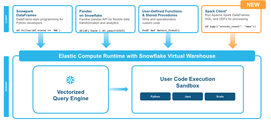
Snowpark Connect expands the developer experience by enabling Spark dataframe and SparkSQL workloads to run on Snowflake engine to achieve significant performance speedups compared to platforms that are usually powered by a hosted Spark engine. To take advantage of Snowflake platform-specific integrations such as Snowflake governance, Cortex AI, Snowflake Intelligence, or pandas, Snowpark continues to offer a suite of easy-to-use tools for developers.
Spark Connect is a client-server architecture introduced in Apache Spark™ 3.4 that decouples the client interface from the Spark execution engine. It allows remote clients to connect to Spark clusters over a gRPC-based protocol. This enables developers to interact with Spark from various languages and environments (i.e., web apps, IDEs, notebooks) without requiring a full Spark or JVM installation on the client side.
At its core, Spark Connect operates by sending logical plans from the client to the server. The server then executes these plans and returns the results. This is achieved through gRPC and protocol buffers (protobufs).
Spark Connect messages are defined using protobuf schemas. These schemas are defined in Spark source code and describe the structure of the logical plans, expressions and results that are exchanged between the client and the server. This standardized message format enables interoperability across different clients and server implementations. For example, take the following Spark code:
# My Spark session is connected to my Snowpark Connect endpoint

df = spark.createDataFrame([(1, 21), (2, 30)], ("id", "age"))
df.show()
Similar to the classic mode of Apache Spark, Spark Connect will continue to build up the underlying query plan until execution is triggered (via e.g., persist, collect, show, etc.). When the show command from above is executed, this is the ExecutePlanRequest (source) that is received by the gRPC server that extends OSS Spark’s SparkConnectServiceServicer (source):
session_id: "8069f6ab-fb2d-4796-8748-fb8998a05aa2"
user_context {
  user_id: "dpetersohn"
}
plan {
  root {
    common {
      plan_id: 2
    }
    show_string {
      input {
        common {
          plan_id: 1
        }
        to_df {
          input {
            common {
              plan_id: 0
            }
            local_relation {
              data: "\377\377\377\377\250\000\000\000\020
                     <binary data continues>
                     \377\377\377\377\000\000\000\000"
              schema: "{\"fields\":[{\"metadata\":{},\"name\":\"id\",\"nullable\":true,\"type\":\"long\"},{\"metadata\":{},\"name\":\"age\",\"nullable\":true,\"type\":\"long\"}],\"type\":\"struct\"}"
            }
          }
          column_names: "id"
          column_names: "age"
        }
      }
      num_rows: 20
      truncate: 20
    }
  }
}
client_type: "_SPARK_CONNECT_PYTHON spark/3.5.6 os/darwin python/3.11.5"
request_options {
  reattach_options {
    reattachable: true
  }
}
operation_id: "20ae08d2-6048-41cb-9c94-d99d34c7bcc8"
At the top level, we have session_id, user_context, plan, client_type, request_options and operation_id. The plan field contains the Spark query plan that was created in the client. Notice that the structure is nested, as a tree.
Let's walk through how this works with a simple "Hello World” example for Spark Connect.
Stating the obvious: The first thing we need if we are going to accept gRPC requests is a gRPC server. How we implement this server is reasonably straightforward: We need to create our own Servicer class that extends SparkConnectServiceServicer (source), then create and add the servicer to a gRPC server we create:
import grpc
from concurrent import futures
import pyspark.sql.connect.proto.base_pb2_grpc as proto_base_pb2_grpc


class MySparkConnectServicer(
    proto_base_pb2_grpc.SparkConnectServiceServicer
):
    # TODO: Override request handlers
    pass


server = grpc.server(futures.ThreadPoolExecutor(max_workers=10))
proto_base_pb2_grpc.add_SparkConnectServiceServicer_to_server(
    MySparkConnectServicer(), server
)
server.add_insecure_port("[::]:15002")
server.start()
server.wait_for_termination()
You can run the above code yourself and connect to it on localhost from a different Python script/repl:
from pyspark.sql.connect.session import SparkSession

spark = SparkSession.builder.remote("sc://localhost:15002").getOrCreate()
df = spark.createDataFrame([(1, 21), (2, 30)], ("id", "age"))
Since we haven’t implemented any request handlers, every request will result in a message that looks like this:
SparkConnectGrpcException: <_InactiveRpcError of RPC that terminated with:
	status = StatusCode.UNIMPLEMENTED
	details = "Method not implemented!"
	debug_error_string = "UNKNOWN:Error received from peer  {grpc_message:"Method not implemented!", grpc_status:12}"
>
With a successful localhost stub implementation, it’s time to start handling the requests properly.
One of the core tenets of the product development was to embrace Spark behaviors. We decided to choose a relatively simple workload to start off with. We landed on this:
df = spark.createDataFrame([(1, 21), (2, 30)], ("id", "age"))
df.show()
print(df.count())
df.select(df.id).show()
df.select("age").show()
df.withColumn(
    "plus1k", df["age"] + 1_000
).select("id", "plus1k").show()
parquet_df = spark.read.parquet("s3://my/bucket/myfile.parquet")
parquet_df.show()
This workload contains:
Creating a DataFrame in the client with lowercase column names
Printing the dataframe content
A group by (df.count)
A column projection with the dot operator (dr.id) and string ("age")
Doing a simple operation on a projected column
Create a new column with the result of the simple operation
Reading a Parquet file from S3
In the interest of keeping this blog post at a manageable length, we will focus on the first two operations: createDataFrame and show. You can use the remaining code as you build your own Hello World Spark Connect implementation.
createDataFrame work in Spark Connect?You may recall that no queries are sent to the server until execution is triggered. The createDataFrame operation is received at the same time as show, since show triggers execution. createDataFrame arrives in the form of a local_relation field in the Relation protobuf (source). The relation field containing the Relation protobuf is contained within the request.plan.root field of the ExecutePlanRequest we receive in ExecutePlan, (technically it is found in the input field of another Relation).
local_relation {
    data: "\377\377\377\377\250\000\000\000\020
            <binary data continues>
           \000\377\377\377\377\000\000\000\000"
    schema: "{\"fields\":[{\"metadata\":{},\"name\":\"id\",\"nullable\":true,\"type\":\"long\"},{\"metadata\":{},\"name\":\"age\",\"nullable\":true,\"type\":\"long\"}],\"type\":\"struct\"}"
}
We have two fields: data and schema. The data field appears to be a string of bytes, and if we look at the Spark source, we get a hint for how to go about deserializing the bytes:
message LocalRelation {
  // (Optional) Local collection data serialized into Arrow IPC streaming format which contains
  // the schema of the data.
  optional bytes data = 1;


  // (Optional) The schema of local data.
  // It should be either a DDL-formatted type string or a JSON string.
  //
  // The server side will update the column names and data types according to this schema.
  // If the 'data' is not provided, then this schema will be required.
  optional string schema = 2;
}
Great! Now we can go about converting the data into an Arrow table by using pyarrow.ipc:
import pyarrow as pa

# rel is the Relation protobuf object referenced above
buffer_reader = pa.BufferReader(rel.local_relation.data)
with pa.ipc.open_stream(buffer_reader) as reader:
    pyarrow_table = pa.Table.from_batches([batch for batch in reader])
Now that we’ve got our data in a pyarrow table, we can easily move it into Snowflake via Snowpark, but there’s also a schema field that we need to account for. In our case, schema is a JSON string. We can use json.loads to convert it into a nested dictionary and then build our own Snowpark schema by mapping the individual types, defined here in their string name (e.g., ”long”) to the Snowpark equivalent. The logic for converting types is omitted because it’s trivial in most cases (but not all!):
import json

snowpark_schema = convert_json_schema(json.loads(rel.local_relation.schema))
With both the pyarrow table and the schema, we can easily create a Snowpark DataFrame:
snowpark_df = snowpark_session.create_dataframe(
    pyarrow_table.to_pandas(),
    snowpark_schema,
)
With the snowpark_df created, we are ready to move on to the df.show() part of the Hello World example.
show work in Spark Connect?df.show() on the Spark client is passed through Spark Connect as a show_string relation object (source). On the server, the show_string relation looks like this:
show_string {
  input {
    ...  # This is the Relation containing the local_relation
  }
  num_rows: 20
  truncate: 20
}
This is pretty straightforward, so let’s take a look at how the Spark Connect client expects the data to be returned. In the pyspark.sql.connect.DataFrame class, we see the following code in _show_string, which is called by show (source):
table, _ = DataFrame(
    plan.ShowString(
        child=self._plan,
        num_rows=n,
        truncate=_truncate,
        vertical=vertical,
    ),
    session=self._session,
)._to_table()
return table[0][0].as_py()
where _to_table returns a pyarrow.Table object. So basically, we need to serialize the string we want to show into an Arrow IPC stream from a 1x1 pyarrow.Table. That’s a pretty elegant way to handle show, since it reuses the Arrow-based transport mechanism already used for other operations (e.g., collect), and this also allows the server to completely control the string formatting.
For the sake of simplicity, we can just use Snowpark’s internal _show_string method to generate the string we want to return (Note: this method is not intended for external use). Then, we can create the required 1x1 pyarrow.Table with the result:
spark_show_string = snowpark_df._show_string()
one_by_one = pa.Table.from_arrays(
    [pa.array([spark_show_string])],
    names=["show_string"],
)
outstream = pa.BufferOutputStream()
batch = one_by_one.to_batches()
with pa.ipc.new_stream(outstream, batch.schema) as writer:
    writer.write_batch(batch)
# Convert to bytes so we can send it over gRPC
show_string_bytes = outstream.getvalue().to_pybytes()
The result is now ready to be passed back from the server by returning an ExecutePlanResponse from the ExecutePlan method on our Servicer object:
import pyspark.sql.connect.proto.base_pb2 as proto_base

yield proto_base.ExecutePlanResponse(
    session_id=request.session_id,
    operation_id=MY_OP_ID,  # The operation id is controlled by the server
    arrow_batch=proto_base.ExecutePlanResponse.ArrowBatch(
        row_count=1,  # Our show string object only has 1 row
        data=show_string_bytes,
    ),
)
At this point our ExecutePlan method looks something like this:
import pyarrow as pa
import pyspark.sql.connect.proto.base_pb2 as proto_base

def ExecutePlan(self, request: proto_base.ExecutePlanRequest, context):
    match request.plan.WhichOneof("op_type"):
        case "root":
            # root is the root Relation protobuf message
            match request.plan.root.WhichOneof("rel_type"):
                case "show_string":
                    # Our hacky hello world example :)
                    rel = request.plan.root.show_string.input.to_df.input
                    buffer_reader = pa.BufferReader(rel.local_relation.data)
                    with pa.ipc.open_stream(buffer_reader) as reader:
                        pyarrow_table = pa.Table.from_batches(
                            [batch for batch in reader]
                        )
                    snowpark_df = snowpark_session.create_dataframe(
                        pyarrow_table.to_pandas(),
                        snowpark_schema,
                    )
                    spark_show_string = snowpark_df._show_string()
                    one_by_one = pa.Table.from_arrays(
                        [pa.array([spark_show_string])],
                        names=["show_string"],
                    )
                    outstream = pa.BufferOutputStream()
                    batch = one_by_one.to_batches()
                    with pa.ipc.new_stream(outstream, batch.schema) as writer:
                        writer.write_batch(batch)
                    # Convert to bytes so we can send it over gRPC
                    show_string_bytes = outstream.getvalue().to_pybytes()
                    yield proto_base.ExecutePlanResponse(
                        session_id=request.session_id,
                        operation_id=MY_OP_ID,
                        arrow_batch=proto_base.ExecutePlanResponse.ArrowBatch(
                            row_count=1,
                            data=show_string_bytes,
                        ),
                    )
                case _:
                    raise NotImplementedError()
        case _:
            raise NotImplementedError()
    yield proto_base.ExecutePlanResponse(
        session_id=request.session_id,
        operation_id=SERVER_SIDE_SESSION_ID,
        result_complete=(
            proto_base.ExecutePlanResponse.ResultComplete(),
        )
    )
This is obviously not the way you’d want to implement this in a production system, but for the sake of the “Hello World” example, this works. If you were to build this yourself, you’d need to be able to parse the whole Spark query plan tree and map the operations to the system you’re implementing it for.
Now that we’ve explored how a “Hello World” example would look, let’s talk in more detail about the architecture of Snowpark Connect for Apache Spark. Figure 2 shows an overview of the architecture.
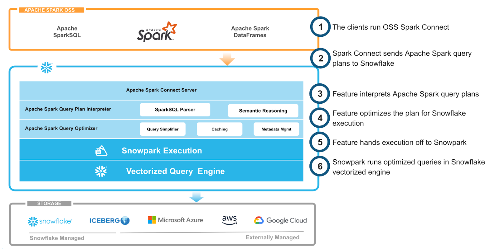
As we mentioned, Spark Connect enables us to implement a server inside Snowflake, such that the user can simply connect to the Snowflake Spark Connect endpoint from their open source Spark installation. How this is done in practice is covered in the getting started docs.
Once Snowflake receives the Spark query plan through Spark Connect, it goes through a series of transformations to create an optimal Snowpark query plan.
One of the most interesting challenges we had to solve was transpiling SparkSQL into Snowflake SQL. We’ll reserve the deep details of the SparkSQL parser for a future post. But in short, our implementation relies on the SparkSQL catalyst parser, and then converts catalyst plans to Spark Connect protobuf. This enabled us to ensure there is only one implementation for each operator necessary, but it also presented some new challenges.
SparkSQL is more expressive than the Spark DataFrame API, meaning that there are multiple SQL operators that are not present in the protobuf definition. Fortunately, Spark developers anticipated the need for extending the Spark Connect protocol, so we use Spark Connect’s extension protobuf for the Relation object for any operators that are in SparkSQL but not in the protobuf definition. Since our parsing logic is all handled server-side, we don’t even need to ship a new client to the user!
This component comprised the majority of the engineering effort. There are several subtle differences between the Snowpark our python client and Apache Spark.
One of the big initial questions was testing. We started by using the open source Apache Spark test suite, thinking that since the open source community uses these tests to check correctness, they would be a good start. Indeed they were very helpful, but there were a lot of other things we needed to consider, since the same assumptions of the open source developers would not hold with the Snowpark engine. Our known compatibility issues are documented here.
In addition to the open source Spark tests, we built a test suite with a combination of hand-written tests (designed to test the edge cases in behavior mismatches between Spark and Snowpark Connect) and AI generated workloads (designed to mirror the types of operations that Spark users write on a daily basis). This testing strategy helped us catch a number of bugs and issues that we might not have been able to catch before Public Preview, particularly in cases where default Spark behavior is undocumented.
Once we built the Spark query plan interpreter, it was simply a matter of letting Snowpark execution handle the optimized query plan we generate via Snowflake’s vectorized query engine. The development of Snowpark Connect for Apache Spark inspired several updates and improvements throughout the stack. For example, improving support for seed-based random samples, performance improvements for complex query plans and more. This architecture effectively brings all of the benefits of Snowflake’s ecosystem directly to Apache Spark users and vice versa.
Snowpark Connect for Apache Spark is now in public preview, try it today! We are continuously working on improving the compatibility gaps with our current coverage against the OSS suite to be at >85% for Snowpark Connect for Spark SparkSQL tests (including HiveSQL and ANSI SQL). Snowflake is hiring for many roles in Product and Engineering. Explore open opportunities and apply today to help build exciting new features like this.