Choosing the Right Jev-Class Model for Your SQL Pipeline
Choosing a classifier starts with the action its answer will trigger. Routing a support request to the wrong team, assigning the wrong sentiment to an earnings-call passage, and missing sensitive information have different consequences. A model that works well for one of those jobs may be a poor choice for another.
Decision models can run natively through Snowflake Cortex AI Functions with Snowflake Decision, currently in private preview. You can also deploy open-weight decision models through Snowflake ML's Model Registry and serve them on Snowpark Container Services (SPCS), subject to their runtime, dependency, hardware, and license requirements. This guide focuses on choosing the model and serving path for your workload.
The recommendations draw on comparisons of Jev, Decider-2B, Laya, Gemini 3.5 Flash, Claude Opus 5 (both called through Cortex AI_COMPLETE), and native AI_CLASSIFY across earnings-call sentiment, banking intents, and sensitive-information detection. Use the findings to build a shortlist, then test that shortlist against your own labels and operating requirements.
Build a shortlist around your workload
"Jev-class" describes decision models that evaluate content against a bounded question and return typed answers and probabilities. TypeSafe's Jev, Decider-2B, and Laya are distinct models in that category. Decider-2B and Laya have open weights you can serve yourself, while the tests reached Jev through a hosted REST API. Their accuracy, stability, and deployment requirements differ.
A useful shortlist also includes alternatives outside that category. A general-purpose LLM may handle difficult cases better, while a managed classification function may meet your requirements without a custom serving stack.
| Workload or requirement | Candidates to evaluate first | What should decide the choice |
|---|---|---|
| Fine-grained intent routing with open weights | Decider-2B; compare Laya on the closest labels | Reference-label match, confusion between neighboring intents, label-order stability |
| Classification in a SQL batch without a custom model service | AI_CLASSIFY alongside your strongest decision-model candidate | Quality gate, full-batch completion time, operational effort |
| Hosted decision inference with external processing permitted | Jev alongside native or self-hosted alternatives | Recall, false positives, integration overhead, data-handling requirements |
| Sensitive-information triage with costly mistakes | Include Opus as a quality baseline | Missed sensitive items and clean items incorrectly flagged |
| Earnings-call sentiment or another subjective labeling task | Compare candidates against a human-reviewed rubric | Independent label quality, ambiguous passages, consistency |
This is a starting point for evaluation, not a ranking across unrelated tasks. The underlying comparisons used frozen text and shared label definitions, without task-specific training during the evaluation. The initial datasets included 200 earnings-call passages from 40 companies and 560 labeled queries from two restricted BANKING77 intent subsets. An expanded study added sensitive-information detection and Jev as a sixth candidate.
For intent routing, test the labels that are easy to confuse
If your pipeline distinguishes closely related payment requests, broad categories such as "billing" and "technical support" won't tell you enough about model quality. Include examples from the neighboring labels that lead to different actions, then inspect those errors directly.
The banking results illustrate why. Laya's reference-label match fell from 95.31% on broad intents to 81.67% on closely related payment intents. When the label list was reversed or shuffled, four of Laya's 60 fine-grained answers changed. Opus changed one of 60, and Decider-2B, Flash, AI_CLASSIFY, and Jev (tested in the expanded study) changed none.
For the harder banking task, the initial comparison reported:
| Candidate | Reference-label match | Median single-row SQL latency |
|---|---|---|
| Decider-2B | 97.08% | 0.393 s |
| Flash | 97.92% | 1.697 s |
AI_CLASSIFY | 96.67% | 0.799 s |
| Opus | 96.67% | 2.096 s |
| Laya | 81.67% | 0.402 s |
If you need open weights, these results make Decider-2B a stronger starting candidate than Laya for fine-grained routing. Laya's broad-intent score alone wouldn't have exposed that weakness. If you don't need to operate your own model, include AI_CLASSIFY before accepting the additional serving work: its quality was close on this task.
Decider-2B's training included BANKING77's training split, while these queries came from the held-out test split. Decider-2B hadn't seen these queries, but it had learned these intents. These restricted-subset results don't establish accuracy on an unseen domain. Before selecting it, repeat the comparison on representative requests from your own application, with independently reviewed reference labels.
The expanded study reported no statistically significant differences among the top five candidates on BANKING77; the only significant differences were between Laya and each of the other five. Treat small differences as uncertain until the test has enough evidence to distinguish them. When several candidates meet your quality requirement, choose among them using the serving and cost requirements below.
For sensitive-information triage, set separate error limits
A classifier used to flag personally identifiable information (PII), protected health information (PHI), or material nonpublic information (MNPI) needs more than an overall accuracy target. Set a limit on missed sensitive items and a separate limit on clean items incorrectly flagged.
Recall measures the fraction of sensitive items detected. The false-positive rate measures the fraction of clean items flagged. Overall accuracy depends on the mixture of sensitive and clean examples, so it can hide an error rate that makes a model unsuitable for your workflow.
The expanded study used a synthetic set of 3,000 items: 1,000 each of table cells, narrative chunks, and JSON records, with equal numbers of PII, PHI, MNPI, and clean items, so three-quarters of the set was sensitive. It reported these results:
| Candidate | Sensitive items caught (recall) | Clean items flagged (false-positive rate) | Exact-label accuracy |
|---|---|---|---|
| Opus | 99.96% | 0.80% | 99.77% |
| Flash | 99.33% | 11.60% | 96.37% |
| Jev | 98.80% | 17.87% | 94.27% |
AI_CLASSIFY | 98.89% | 32.40% | 90.83% |
| Decider-2B | 60.89% | 18.40% | 65.83% |
| Laya | 11.91% | 8.00% | 31.67% |
All of AI_CLASSIFY's false positives came from clean items built to look sensitive, and it gave the same label to every pair in which only the table context differed.
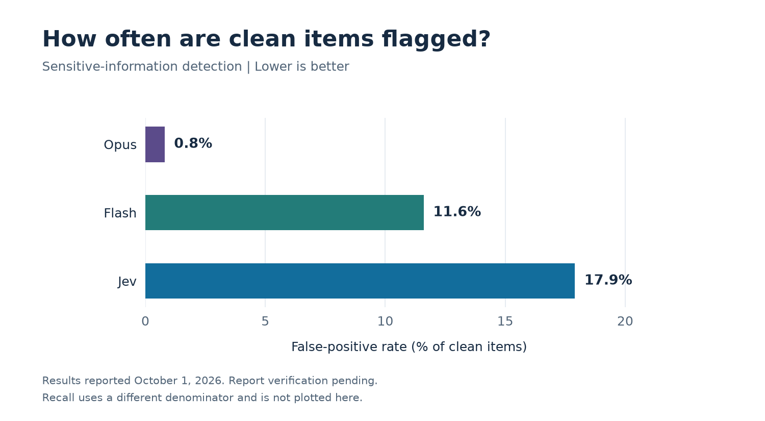
Those results suggest different uses. Jev is a candidate for high-recall triage if the downstream process can tolerate its review volume. Include Opus when unnecessary flags are expensive or when the quality target is stricter. Opus's additional expense bought a quality improvement on this workload, unlike in the initial banking comparison, which didn't establish a quality advantage that justified its premium.
Estimate the downstream effect with your actual traffic mix. A false positive that adds a record to a review queue has a different cost from one that blocks a transaction. Evaluate those consequences before deciding that the less expensive model call produces the less expensive pipeline.
These classification results don't establish a certified compliance control or justify automatically releasing records that a model labels clean.
For sentiment analysis, validate the reference before ranking models
Earnings-call sentiment introduces a different selection problem: what should the label mean? A passage can describe weaker current results and an optimistic forecast. Your rubric needs to specify which aspect to classify and how to handle mixed or uncertain language.
Start with human-reviewed examples that make those distinctions explicit. If one model supplies the reference answers, agreement with that model measures consistency with the reference, not independent accuracy. Keep that distinction in your results table.
The earnings passages had no reference labels by design, so the comparison measured agreement between models, not accuracy. All six models agreed on 93 of 200 passages, and Laya labeled 142 of 200 positive, far more than the others. Use this workload to evaluate rubric adherence and disagreement cases rather than carry over the banking ranking.
For your own pipeline, keep the rubric fixed across candidates and have reviewers examine disagreements without seeing which model produced each answer. Resolve unclear label definitions before attributing every disagreement to model quality.
Choose a serving path for latency or batch throughput
Once a candidate meets the quality gate, measure it through the interface your pipeline will use. An interactive application needs request-to-response latency. A scheduled SQL pipeline needs full-batch completion time. Model-only timing doesn't determine either result.
On the harder banking task, AI_CLASSIFY processed 240 queries in 7.38 seconds, compared with Decider-2B's 13.22 seconds. Laya, running on the same A10G GPU as Decider-2B, took 7.41 seconds.
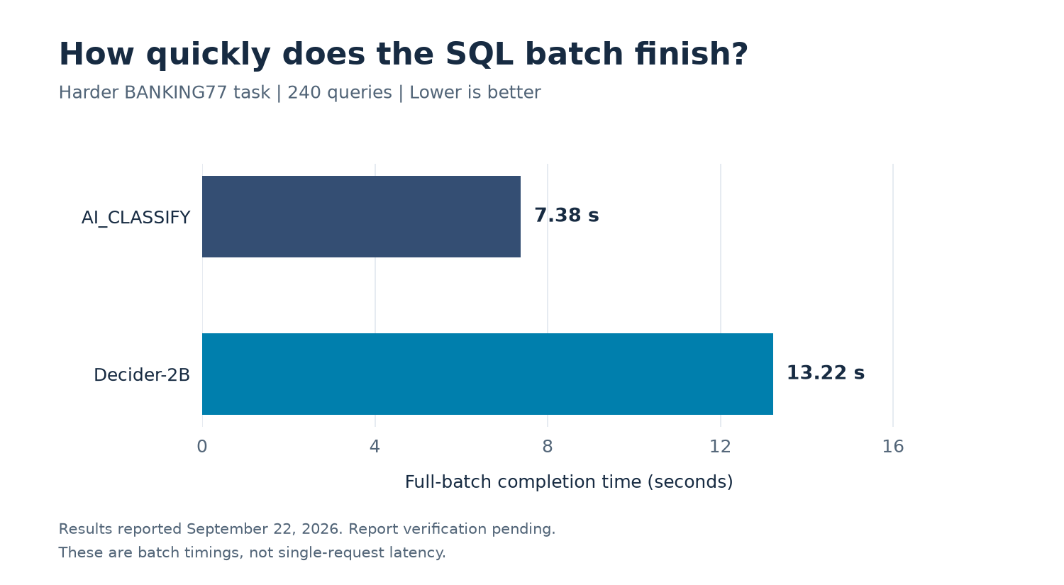
Initial comparison: one full-batch run per model on September 22, 2026, on an X-Small warehouse. The GPU service processed each request batch row by row on one A10G, so these aren't optimized serving numbers or single-request latencies.
Jev, tested in the expanded study through its external API route, took 5.59 seconds, the fastest of the six candidates.
A low single-row latency didn't make Decider-2B the fastest SQL batch. For a batch-oriented workflow, test the managed classification path before taking on a custom serving stack solely for speed.
The external Jev integration further illustrates the effect of the serving path. Its API call time was reported at approximately 0.2 seconds, while single-row SQL calls took approximately 3.8 seconds through a Python UDF. The overhead was attributed to starting the UDF for each call. BANKING77 batches through that integration achieved 43–51 rows per second.
That SQL integration is a candidate for batch evaluation, but its API timing alone would be a poor basis for an interactive latency target. The UDF measurements also shouldn't be applied to an SPCS REST endpoint or every possible Jev integration. The earlier post used a different path for its real-time application measurements.
Match inputs, batch sizes, concurrency, and timing boundaries when testing your shortlist. Run multiple repetitions, report warmups separately, and retain slow calls and failures. Record the model identifier and run date so the result describes a reproducible configuration rather than an assumed property of the model.
| Deployment choice | Advantages | Disadvantages |
|---|---|---|
| Open-weight models on SPCS | Choose the model and control its packaging, GPU capacity, and serving configuration. | You operate the service and manage scaling; startup and idle GPU time add cost. |
Native AI_CLASSIFY | Call directly from SQL without managing a GPU service; faster than Decider-2B on the tested 240-query SQL batch. | Uses a managed model rather than your chosen open-weight model; its median single-row latency, approximately 0.8 seconds, was about twice Decider-2B's. |
| Jev through the tested external API route | Hosted inference without managing model-serving GPUs; approximately 0.2-second API calls in the test. | Inputs leave Snowflake; gateway and UDF integration add work, and the tested SQL path increased single-row latency to approximately 3.8 seconds. Provider terms and rate limits also apply. |
The tested Jev route sent inputs outside Snowflake through Vercel AI Gateway. If external processing is allowed, review the provider's terms and your organization's requirements before sending production data. If your requirements rule out that route, evaluate native functions and self-hosted alternatives instead.
Compare operating costs after the quality gate
Compare costs among candidates that can do the job acceptably. A low inference price won't compensate for an error rate that makes the workflow unusable, and a more expensive model may not improve quality on the task you need.
The BANKING77 costs included allocated operating overhead:
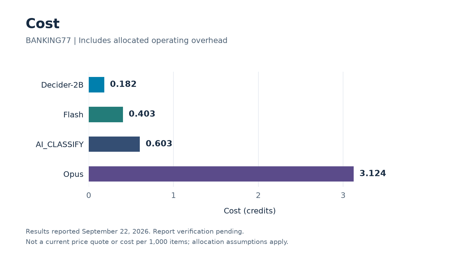
Laya cost the least, approximately 0.156 credits, but it was also the least accurate candidate on the fine-grained intents. For this banking workload, the costs support evaluating Decider-2B before defaulting to Opus. These are experiment totals under the original allocation assumptions, not current price quotes or costs per 1,000 items. Startup, idle time, and failed calls affected those totals.
Open weights still require compute. A service may accrue GPU costs between requests; a batch job may spend time starting before processing its first row. Native function usage, warehouse execution, and external API charges contribute differently depending on the serving path.
In the expanded study, the gateway-reported charges for Jev's 4,729 calls ($0.112) were consistent with the Vercel usage page ($0.11), and none of the calls failed or needed a retry. That establishes an external API cost component, not the full cost of the surrounding UDF and warehouse. It shouldn't be compared directly with an infrastructure-inclusive total from another experiment.
For your estimate, separate model/API usage, warehouse execution, serving capacity, and allocated startup or idle time. State which components are measured and which are estimated. If flags create manual work, add a separate review-cost assumption based on your traffic and error rates. Use a common denominator, such as correctly processed items at the required service level, when comparing qualifying candidates.
Validate your selection on a held-out workload
Turn the shortlist into a selection by setting acceptance criteria before tuning it. Define what a wrong answer costs, how quickly results must arrive, and which deployment routes are permitted. Then use the same evaluation procedure for each candidate:
- Freeze a representative, independently labeled test set. Include ambiguous cases and labels that trigger different downstream actions.
- Fix the label definitions and preserve prompts, versions, and raw responses. Track invalid answers separately from valid but incorrect ones.
- Measure the relevant quality gates: per-label errors for routing, rubric agreement for sentiment, and recall plus false positives for sensitive-information triage. Check repeatability and label-order sensitivity.
- Benchmark the qualifying candidates through the intended serving path, using matched batching and concurrency. Include the operating costs that path actually incurs.
- If you adjust prompts or probability thresholds, use a separate held-out set for the final decision. Recheck the chosen configuration when the model or workload changes.
Decision-model probabilities can support a later escalation policy for uncertain cases. Calibrate those probabilities against your workload before treating a threshold as a reliability guarantee, and evaluate any cascade with both stages' costs and errors included.
For deployment details, see the earlier post, which covers Model Registry and SPCS. For a managed SQL baseline, start with the AI_CLASSIFY documentation and evaluate which other candidates can maintain your required accuracy bar at lower cost.
This content is provided as is, and is not maintained on an ongoing basis. It may be out of date with current Snowflake instances
