

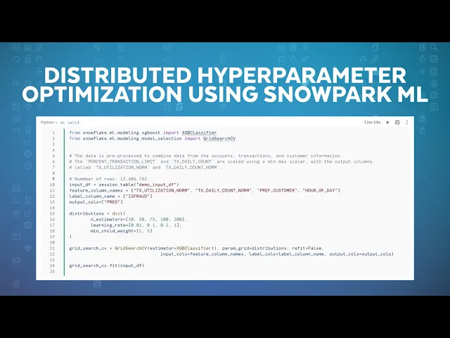
Hyperparameter Tuning: How to Spend a Search Budget Well
Learn how to prioritize hyperparameters, define an efficient search space, allocate compute across trials and recognize when further tuning no longer justifies its cost.
HYPERPARAMETER TUNING DEFINED
Hyperparameter tuning, also called hyperparameter optimization, searches for the configuration settings that produce the strongest model performance under a defined evaluation method and resource budget.
Each hyperparameter search makes a set of bets: that the settings being tested will affect model performance, that the chosen ranges contain better options, that the evaluation will detect real improvement and that another run is worth the time and cost required. The search algorithm determines which configuration to try next, but it can’t make those underlying choices for us.
A poorly chosen search space directs trials toward implausible configurations. Repeated use of the same validation data increases the risk of selecting for statistical noise. Large searches magnify data-loading overhead and infrastructure costs, while increasing the likelihood of testing configurations that exceed available memory. Algorithm choice, search-space design, evaluation, and resource allocation must be considered together.
At its best, hyperparameter tuning is a disciplined way to allocate a finite model training budget. The process should concentrate resources where performance is most sensitive, evaluate each candidate under a sound protocol and stop when the expected gain no longer justifies its statistical and operational cost.
What is hyperparameter tuning?
Hyperparameter tuning, also called hyperparameter optimization (HPO), searches for the configuration settings that produce the strongest performance of a machine learning model under a defined evaluation method and resource budget. These settings might include the learning rate, batch size, number of layers or regularization strength.
Hyperparameters differ from model parameters in how they’re determined. The training algorithm learns model parameters, such as neural network weights, from the training data. Hyperparameters are supplied by practitioners or tuning software and shape how that learning process works.
How hyperparameter tuning works
A typical search follows an iterative loop. First, the tuning process selects a configuration from a defined search space. It then trains a model, scores the result on validation data and records the configuration alongside its metrics. Depending on the search strategy, that result may inform the next configuration. The process continues until it reaches a trial limit, exhausts its compute budget or satisfies another stopping condition.
Many workflows also compare model families or architectures during the same experiment. Statistically, those comparisons belong to the same model-selection process as hyperparameter tuning — both use validation evidence to choose among candidates.
Hyperparameter tuning can’t compensate for poor labels, weak features, insufficient data or an unsuitable model family. Those problems often set a harder limit on performance than any choice of configuration. Once the team has developed a sound baseline model, however, structured tuning can help identify a better-performing configuration and provide a record of what was tested so the results can be reproduced.
Watch Chase Romano, Data Scientist at Snowflake, demonstrate how to tune hyperparameters and turn them into objects that can then be fed into your model for optimized performance:
How to design an efficient hyperparameter search
Most models have more configurable settings than a team could practically explore. Efficient tuning begins by narrowing the field, then defining ranges and sampling methods that reflect how each setting behaves.
Prioritize influential hyperparameters
Not every hyperparameter deserves the same amount of attention. Teams usually start with the settings most likely to affect validation performance, training stability or computational cost. For neural networks, that often means looking first at the learning rate, then at related choices such as batch size, regularization and model capacity.
Other model families tend to be more sensitive to different settings:
| Model family | Common high-impact hyperparameters |
|---|---|
| Neural networks | Learning rate, batch size, regularization, dropout and capacity |
| Decision trees | Maximum depth, minimum samples per leaf and split criterion |
| Random forests and other bagged tree ensembles | Number of estimators, maximum depth, minimum samples per leaf, maximum features and sampling settings |
| Gradient-boosted trees | Learning rate, number of boosting rounds, tree depth or leaf complexity, subsampling and column sampling |
| Support vector machines | C, kernel and gamma |
These priorities are just a starting point. A small preliminary search can help show which settings actually influence the results for a particular model and data set. Teams can then explore those dimensions more broadly while leaving less sensitive settings near reasonable defaults. Closely related settings, such as learning rate and batch size, are usually more useful when evaluated together rather than interpreted on their own.
Design the search space deliberately
A search space defines which hyperparameters the optimizer will consider, which values each one can take, how those values will be sampled and how each trial will be scored. Together, those choices determine what the optimizer can realistically find. For example, a simple search space might allow a learning rate between 0.0001 and 0.1 and a batch size of 32, 64 or 128. Each trial selects one combination from those possibilities.
If the ranges are too narrow, the search may exclude strong configurations. When the best trials cluster at the upper or lower boundary, that often suggests the range stopped too soon. A range that is too broad creates the opposite problem: The optimizer spends trials in regions that practical experience suggests are unlikely to work well.
The sampling distribution matters just as much as the range itself. Learning rates and regularization values often vary by factors of 10 rather than by fixed increments. For this reason, logarithmic sampling gives small and large values a fairer chance of being tested. For example, a search from 0.0001 to 0.1 should explore values around 0.0001, 0.001, 0.01 and 0.1 rather than concentrating most trials near 0.1.
Discrete choices work well for settings such as kernel type or optimizer family, while conditional spaces avoid testing irrelevant combinations. A momentum value, for example, only needs to appear when the selected optimizer actually uses momentum.
The scoring objective also needs attention. Accuracy can hide weak performance on a minority class in an imbalanced classification problem, while low validation loss may say little about production constraints such as latency or memory use. When several criteria genuinely matter, teams can evaluate them together rather than forcing everything into a single score. This makes trade-offs visible — for example, one configuration may be slightly more accurate while another is much faster or uses less memory.
Leaving a setting at its default may be completely reasonable. Recording that decision, along with the ranges used for the settings that were tuned, makes it clear which choices were intentional and which variables simply went unexamined.
QUICK TIP
Start with fewer hyperparameters and wider, well-reasoned ranges. Early results will usually tell you more about which dimensions deserve attention than a large search across every available setting.
Match the search strategy to the trial economics
A team testing a few discrete settings may be able to evaluate every possible combination, but as the number of hyperparameters grows, that approach quickly becomes impractical. Teams choose a search strategy based on the specifics of the trial.
- Grid search: Grid search works through every combination in a predefined set of values. It’s easy to understand and reproduce, which makes it useful for small search spaces with only a few discrete choices. The number of trials grows rapidly as more settings are added, however, and much of that work may go toward hyperparameters that have little effect on performance.
- Random search: Random search samples configurations independently instead of testing every combination. With the same trial budget, it usually explores more distinct values across each hyperparameter. In their landmark study, James Bergstra and Yoshua Bengio found that only a few hyperparameters drove performance on most data sets, giving random search broader coverage of the settings that mattered than grid search at the same trial budget. Because each trial can run independently, random search also works well with parallel compute.
- Bayesian search: Bayesian optimization uses the results of earlier trials to decide what to test next. It builds an estimate of how different configurations are likely to perform, then favors settings that appear promising while still exploring uncertain parts of the search space. This can reduce the number of evaluations needed when each training run is expensive. The method adds overhead, however, and becomes harder to use efficiently when many trials run at the same time.
- Population-based search: Population-based training changes hyperparameters while training is already underway. It runs several models concurrently, keeps stronger performers and adjusts their settings over time. This makes it useful for finding schedules, such as a learning rate that changes during training, but it also requires more compute and orchestration than the other methods.
For many projects, random search is a practical place to start because it scales well and is easy to parallelize. Grid search fits small, discrete spaces, while Bayesian optimization is more useful when trials are costly and earlier results can guide later ones. Population-based training is generally reserved for cases where changing hyperparameters during training is worth the added complexity.
Use early results to allocate training
Training every configuration to completion can waste substantial compute on trials that show little promise. Early-stopping methods address that problem by giving each trial a limited initial budget, then directing more resources toward the configurations that perform best.
Successive halving, Hyperband and ASHA all follow the same broad principle: spend a small amount of compute on many candidates, stop weaker trials early and devote more resources to the ones that remain promising.
- Successive halving: Successive halving starts with many configurations and trains each one using a small resource allocation, such as a limited number of epochs or training examples. It then keeps the strongest performers, drops the rest and gives the surviving trials a larger budget. Repeating that process gradually concentrates compute on the most promising candidates.
- Hyperband: Hyperband applies the same basic idea across several schedules. Some schedules begin with more configurations and smaller budgets, while others test fewer configurations more thoroughly from the start.
- ASHA: Asynchronous Successive Halving Algorithm (ASHA) removes the need for workers to advance in lockstep. As soon as a trial produces enough evidence, the system can promote or stop it without waiting for every other trial in the same round to finish. This helps keep workers busy when training times vary.
These methods work best when early results provide a useful signal about eventual performance. That assumption doesn’t always hold. Some configurations improve slowly, and learning curves may cross later in training, so aggressive pruning can eliminate a trial that would eventually perform well. Teams still need to decide how much training a trial receives before it can be stopped and how aggressively weaker trials should be eliminated.
Plan for infrastructure constraints
A search over 50 configurations represents roughly 50 training jobs, reduced only when pruning ends some of them early. If one complete run takes an hour, running the trials sequentially requires about 50 hours of training. Concurrency speeds up the search, but it doesn’t remove the underlying compute cost.
As the workload grows, infrastructure can become the limiting factor. Training jobs compete for data-pipeline capacity, CPUs or GPUs and scheduler availability. Adding more parallel trials only helps when the underlying system can keep those jobs supplied with data and compute.
Teams can manage that pressure by limiting concurrency, scheduling trials according to their resource needs and reusing preprocessing results where it is safe to do so.
Memory may narrow the search as well. Larger models, wider batches or higher-resolution inputs can exceed a worker’s capacity before producing a result. Teams can exclude configurations that exceed known hardware limits, treat out-of-memory failures as invalid trials and use smaller proxy runs to screen expensive candidates. The leading configurations should still be verified at full scale, however, because rankings don’t always carry over from reduced data, model size or input resolution.

How to avoid the validation trap
A tuning process chooses the configuration with the best validation score. Even when the candidates would perform similarly on the broader population, random variation in a finite validation sample will make some look better than others. The more configurations a team tests, the more likely it is to select one that benefited from unusually favorable variation.
Repeatedly tuning against the same validation set deepens that effect. Decisions such as widening a search range, changing the model family or launching another round of experiments all incorporate information from the validation results. Over time, the development process begins adapting to patterns specific to that data, even though the model is never trained directly on those records. Research on model-selection bias has shown that repeatedly optimizing against the same evaluation evidence can make apparent performance differences look more meaningful than they really are.
With enough data, teams can reduce that risk by assigning each split a distinct role:
- The training set fits the model parameters.
- The validation set selects hyperparameters and models.
- The untouched test set estimates final performance on new data.
The test set should be used for one final evaluation. Once its result influences another tuning decision, it effectively becomes part of the validation process and no longer provides an independent estimate.
For smaller data sets, teams may use nested cross-validation to separate tuning from evaluation without reserving a large permanent test set. One set of folds is used to choose configurations, while a separate held-out fold evaluates the resulting selection process.
Preprocessing steps must be kept inside the same training and validation boundaries as the model itself. A scaler, for example, calculates statistics from the data it receives. If it’s fitted before cross-validation, those statistics include records that will later appear in the validation folds, allowing information from the held-out data to influence training indirectly. Imputation, feature selection, encoding and resampling can create the same problem. Fitting the entire pipeline separately within each training fold prevents that leakage.
The final metric should describe how the full model-selection process performs on unseen data, not simply report the highest validation score observed during tuning. That distinction becomes increasingly important as teams compare more models, features and configurations against the same evidence.
COMMON PITFALL
A common mistake is treating the validation set as an unlimited source of feedback. Each new search round adapts the development process more closely to that data, increasing the chance that the selected configuration benefited from noise.
When should you stop tuning?
A fixed trial count gives a search a clear budget, but it doesn’t account for whether the team has explored the space adequately. Fifty trials may be enough for a small search space but barely begin to cover a larger one. A good stopping decision looks at whether performance is still improving, whether the leading results are meaningfully different and whether another round of tuning is worth the cost.
Is performance still improving?
Strong gains often appear early in a search, followed by smaller improvements as the search continues. When new trials stop improving the best result and the leading configurations cluster within a narrow range, further tuning may offer limited value. What counts as a meaningful difference depends on both statistical uncertainty and the use case. A 0.5% improvement could justify substantial compute for a high-volume fraud model, for example, while a larger gain may have little practical effect in a low-frequency internal workflow.
Are the leading results meaningfully different?
The apparent difference also needs to hold up across repeated runs. A configuration that leads by a small margin but varies widely across folds or random seeds provides weaker evidence than a slightly lower-scoring candidate that performs consistently. Rerunning the strongest configurations several times with different random seeds can show whether the ranking reflects a persistent advantage or favorable randomness. Random seeds affect sources of variation such as weight initialization, data shuffling and sampling, so two runs with the same hyperparameters may not produce exactly the same result.
Is another round of tuning worth the cost?
Teams should then compare the likely return from more tuning with other uses of the same budget. Correcting label errors, adding training data, investing in feature engineering or selecting a more suitable model family may improve performance more than another search round. Tuning is most useful when those foundations are already sound and configuration choices still appear to be the limiting factor.
It’s also important to note that cost includes more than compute. Data preparation, orchestration, failed runs and experiment review all consume engineering time. For example, the same measured gain carries a different value when it requires two unattended GPU hours than when it requires two engineers to investigate unstable runs for a week.
Production requirements may narrow the choice further. The configuration with the highest validation score may still exceed latency, memory or training-cost limits. Evaluating those criteria during the search helps teams identify configurations that are both accurate enough and practical to deploy.
The goal isn’t to prove that no better configuration exists, but to gather enough evidence that further tuning no longer deserves priority over the team’s other options.
Hyperparameter tuning on Snowflake
In practical terms, the workflow has four parts: define the configurations to test, run those training jobs against data, compare their results and retain the selected model and its metadata.
Within Snowflake ML Container Runtime, the Hyperparameter Optimization API provides a model-agnostic framework for parallel tuning. Teams define a search strategy, sampling distributions and training function, then use the Tuner interface to run trials against Snowflake data. The API supports Snowflake ML modeling APIs as well as open source frameworks.
Parallel execution addresses one side of the cost equation. Trials run in Container Runtime on Snowpark Container Services compute, where available CPU or GPU resources support concurrent training. For larger individual models, Container Runtime also provides distributed training APIs for frameworks including PyTorch, XGBoost and LightGBM.
Data access shapes the other side of the equation. Training directly against governed Snowflake data reduces the separate extraction and transfer workflows that often sit between source tables and model-development infrastructure. Because every trial needs access to training data, reducing repeated data movement can save time and operational overhead across a large search. Snowflake ML also supports open source code and libraries for model development, allowing teams to preserve existing training approaches while working near the data.
Once the trials finish, Snowflake ML Experiments organizes training runs for comparison, while the Model Registry stores models and associated metadata for subsequent management and inference. Together, those capabilities preserve the relationship among a configuration, its evaluation results and the model selected from the search.
Teams retain the run history used to justify the selection. Compute, governed data and experiment metadata remain connected as the model moves toward registration and deployment.
Make tuning a defensible engineering decision
The goal of hyperparameter tuning is a configuration whose advantage holds up under evaluation and makes sense for the workload. To achieve this goal, teams need to decide which settings belong in the search, define credible ranges, choose an objective that reflects the real task and set a budget before the first trial runs.
The search method should follow the economics of the experiment, but its value depends on the surrounding design: a sound validation protocol, production constraints established in advance and a stopping rule tied to meaningful improvement.
The selected model should therefore come with more than a winning score. Its record should show what the team tested, how the candidates were evaluated, what the search consumed and why further tuning no longer justified the cost. That evidence turns the final configuration into a reproducible engineering decision.
KEY TAKEAWAY
Hyperparameter tuning is less about finding the perfect search algorithm than deciding where limited compute will create the most value. A focused search space, sound evaluation protocol and clear stopping rule matter more than running the largest possible experiment.
Frequently Asked Questions
Your common questions about hyperparameter tuning, answered by Snowflake experts.
How many hyperparameter-tuning trials are enough?
No fixed number fits every search. Set a resource budget in advance, then track whether additional trials continue to improve the objective by a practically meaningful amount. The size of the search space, cost per run and variation among repeated evaluations provide better guidance than a universal trial count.
Is hyperparameter tuning the same as automated machine learning?
No. Hyperparameter tuning searches for configurations within a defined modeling workflow. Automated machine learning (AutoML) may cover a broader sequence that includes data preprocessing, feature handling, algorithm selection and tuning. HPO may operate independently or as one component of an AutoML system.
Explore AI Resources
Explore AI Topics
Deep dives into every aspect of artificial intelligence
