Oct 5, 2026/5 min readData Engineering
Dynamic Tables with Aggregates Just Got More Price-Performant


Aggregation pipelines are one of the most common patterns we see among Dynamic Tables customers: rollups of orders to the customer, sessions to the account, sensor readings to the device. Define the GROUP BY in a Dynamic Table and the pipeline stays fresh automatically. No refresh logic to write.
Snowflake has made this pattern meaningfully faster. For supported aggregates at the top of a Dynamic Table's definition, Snowflake now refreshes by building on the values already stored instead of recomputing affected groups from scratch.
It’s automatic — there is no new keyword and no option to set. The improvement applies on its own when a definition has the right shape. What follows is how that works:
The part of incremental refresh that isn't obvious
Take a Dynamic Table that keeps a running total of energy consumption as well as the peak reading per meter:
CREATE OR ALTER DYNAMIC TABLE dt_meter_consumption
  TARGET_LAG = '5 minutes'
  WAREHOUSE = pipeline_wh
AS
  SELECT
    meter_id,
    SUM(kwh) AS kwh_total,
    MAX(kwh) AS kwh_peak
  FROM meter_readings
  GROUP BY meter_id;
In theory, this query should be incrementalizable and price-performant. Only a small slice of meter_readings changed, so surely only a small slice of work follows.
The first half of that is true. If 100 new readings arrive and they belong to 40 meters, only 40 groups are affected while the other many-million or so are untouched and can be left alone. Narrowing the work to just the affected groups is the easy win. Dynamic Tables has always done this.
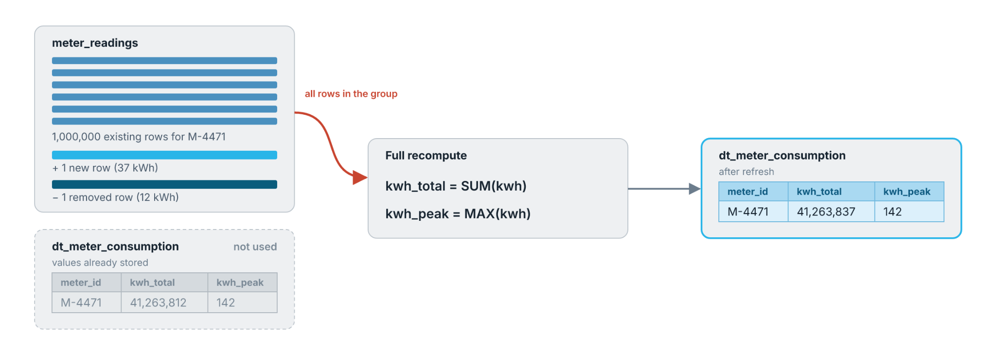
The second half is where it gets tricky. Knowing which groups changed is not the same as knowing their new values. An aggregate is computed over every row in its group, so the straightforward way to get a new value is to read the group's rows and compute it again. That means a single new reading for a meter with a million historical readings pulls all million of them back through the computation. The change was one row; the bill was the whole group.
That is the asymmetry that Dynamic Tables had until recently: Work used to scale with the size of the affected groups, not with the size of the change that affected them.
Building on what's already there
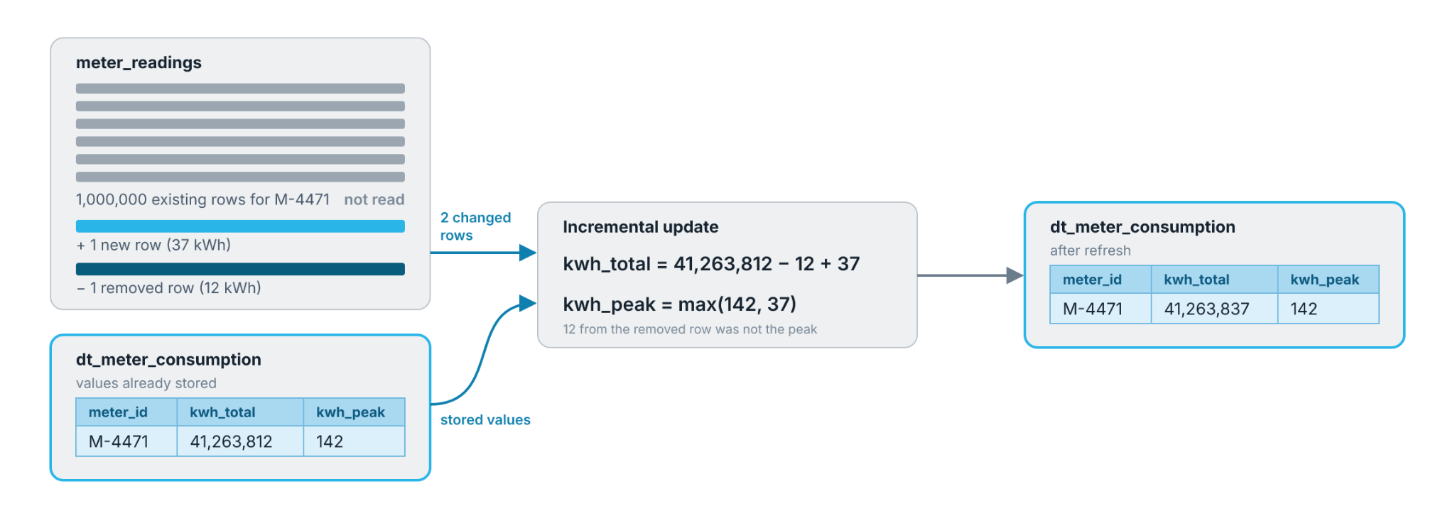
The insight is that the Dynamic Table already holds the answer from its last refresh. If a meter's total was known then, and one reading has since arrived, the new total does not require revisiting years of history.
That is what Snowflake now does. For a qualifying definition, refresh reuses the values already stored in the Dynamic Table and carries them forward using only the rows that actually changed. Work scales with the size of the change, not with the size of the groups it lands in.
How this works depends on the aggregate function. A SUM is the simplest case, because the new value is just arithmetic on the old one:
newSum = oldSum + insertedSum - deletedSumThis translates into: whatever was stored, plus what arrived, minus what left — and not a single source row read. Counts behave the same way, and anything Snowflake derives from sums and counts inherits the benefit: averages and the standard deviation and variance family among them.
A MAX behaves the same way as long as rows only arrive: a new reading either beats the stored peak or it doesn't, so the new value is max(oldPeak, insertedPeak).
Deletions are the harder direction, because not every aggregate is invertible. For a SUM it is just the subtraction in the formula: remove a duplicate reading of 12 kWh from meter_readings and the total adjusts by exactly that. But take a MAX whose current maximum gets deleted. The stored value is gone, and the replacement could be any of the million other rows in the group, so carrying it forward is not enough on its own. Snowflake spots cases like this and recomputes the aggregates — but only for the groups that need it, while every other group still benefits from the new optimization.
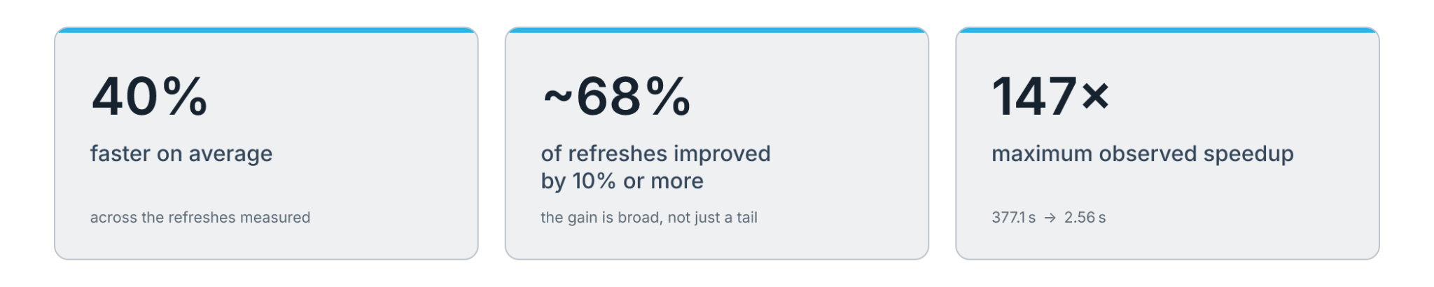
The order of magnitude of performance improvement depends on the aggregate and on how the changes land, but the effect is substantial. Our internal measurements cover Dynamic Tables with a top-level GROUP BY that qualify for this optimization, and are limited to refreshes that previously took more than 3 seconds. Total refresh duration fell by about 40% on average, and more than two-thirds of those refreshes improved by at least 10%. The largest single improvement we saw was 147x: a refresh that had taken roughly 377 seconds finished in about 2.5 seconds.
When a join sits on top of the aggregate
The structural requirement is placement: the GROUP BY needs to be the top-level operation of the Dynamic Table. Anything stacked above the aggregate disables the optimization (for example, a join or a union). A HAVING clause is supported, because it belongs to the grouping.
Consider a table tracking energy readings per meter, enriched with details about the site each meter belongs to:
CREATE OR ALTER DYNAMIC TABLE dt_site_consumption
  TARGET_LAG = '5 minutes'
  WAREHOUSE = pipeline_wh
AS
  SELECT
    s.site_name,
    s.tariff_band,
    m.kwh_total,
    m.kwh_peak
  FROM (
    SELECT meter_id, SUM(kwh) AS kwh_total, MAX(kwh) AS kwh_peak
    FROM meter_readings
    GROUP BY meter_id
  ) m
  JOIN dim_sites s ON m.meter_id = s.meter_id;
The aggregate is buried in a subquery with a join above it, so the GROUP BY is not the top-level operation and the definition does not qualify.
Splitting the two responsibilities across a pair of Dynamic Tables fixes it. The first does nothing but aggregate; the second joins on top of the result:
CREATE OR ALTER DYNAMIC TABLE dt_meter_consumption
  TARGET_LAG = DOWNSTREAM
  WAREHOUSE = pipeline_wh
AS
  SELECT
    meter_id,
    SUM(kwh) AS kwh_total,
    MAX(kwh) AS kwh_peak
  FROM meter_readings
  GROUP BY meter_id;

CREATE OR ALTER DYNAMIC TABLE dt_site_consumption
  TARGET_LAG = '5 minutes'
  WAREHOUSE = pipeline_wh
AS
  SELECT
    s.site_name,
    s.tariff_band,
    m.kwh_total,
    m.kwh_peak
  FROM dt_meter_consumption m
  JOIN dim_sites s ON m.meter_id = s.meter_id;
Now the aggregates have a Dynamic Table of their own, with the GROUP BY on top and the key and both aggregates plainly selected, so it qualifies. TARGET_LAG = DOWNSTREAM lets it refresh its consumer needs on the schedule, and the join moves to a table which only does the job of joining. As a bonus, the aggregated result is now available to anything else that needs it.
Getting the benefit
Dynamic Tables with top-level aggregates just got even more price-performant. Check out the Dynamic Tables refresh optimization documentation to make sure your own Dynamic Tables benefit from this optimization.
