Build Your First ML Model in Snowflake with Agentic ML

Snowflake for Developers/Guides/Build Your First ML Model in Snowflake with Agentic ML

Quickstart

Build Your First ML Model in Snowflake with Agentic ML

Sho Tanaka, Caleb Baechtold, Lucy Zhu

1. Overview

Snowflake ML is changing how teams work with agentic ML, an autonomous, reasoning-based system that enables developers to use agents to plan and execute tasks across the entire ML pipeline. In this quickstart, learn how to build and run a customer lifetime value (LTV) prediction model with only a handful of prompts so that you can go from raw data to production predictions in minutes, not weeks, with Cortex Code, Snowflake's AI native coding agent. Cortex Code is available both as a CLI and directly in Snowsight, Snowflake's web interface.

Important: Cortex Code is powered by LLMs and is non-deterministic. The code it generates may differ from what is shown in this guide. Always review the output and verify that the results match your expectations before proceeding to the next step.

What You'll Learn

Generate realistic synthetic e-commerce data with natural language prompts
Perform exploratory data analysis and feature engineering conversationally
Train and compare multiple regression models inside Snowflake
Log models with metrics to the Snowflake Model Registry
Run batch inference on a Snowflake Warehouse
(Optional) Deploy a model as a REST API on Snowpark Container Services (SPCS) for real-time inference

What You'll Build

A complete customer LTV prediction pipeline featuring:

Synthetic e-commerce transactions dataset (~500 customers, ~100,000 transactions over 18 months)
Trained regression model predicting a customer's total spend in the next 90 days
Registered model in the Snowflake Model Registry with evaluation metrics
Batch inference predictions via Snowflake Warehouse
(Optional) A real-time inference REST endpoint on SPCS with latency profiling

Prerequisites

Sign up for the 30-day free trial of Snowflake. Have ACCOUNTADMIN role or a role with permissions to create databases, schemas, tables, and models
Cortex Code in Snowsight (no local installation required)
A dedicated Snowflake warehouse
(Optional for SPCS) A compute pool configured for Snowpark Container Services — see the official setup guide
Familiarity with basic ML concepts (training, evaluation, inference)

Using Cortex Code CLI? The same prompts work in both interfaces. See Cortex Code CLI Walkthrough for CLI-specific setup and terminal output examples.

2. Setup

Cortex Code in Snowsight

Cortex Code is an AI agent built into Snowflake, designed for data engineering, analytics, ML, and agent-building tasks. It operates autonomously within your Snowflake environment, leveraging deep knowledge of RBAC, schemas, and platform best practices.

Open a Workspace Notebook by going to the sidebar and clicking on Projects > Workspaces; then in the "My Workspace" panel, click on "+ Add new" > Notebook.
Once the notebook loads, look for Cortex Code in the lower-right corner of Snowsight.

Note: Cortex Code is environment aware so using it in a Workspace Notebook will give the best results as it will have access to all the tools provided by the notebook. When relevant, generated code will be inserted into the notebook and run on your behalf.

You are now ready to start prompting Cortex Code to build your ML pipeline.

3. Generate Synthetic Data

First, let's create the database objects and generate synthetic e-commerce transaction data using Cortex Code.

Prompt

Generate realistic looking synthetic data in database COCO_DB and schema COCO_SCHEMA 
(create if it doesn't exist). Create a table ML_LTV_TRANSACTIONS
with ~100000 transactions from ~500 customers over an 18-month period. Include
CUSTOMER_ID, TRANSACTION_TIME, AMOUNT, PRODUCT_CATEGORY, and CHANNEL. Make the
data realistic: customers should have varying purchase frequencies (some buy
weekly, others monthly), amounts should vary by category (electronics $50-$2000,
groceries $10-$200, apparel $20-$500), and channels should be web, mobile, or
in-store. About 10% of customers should be high-value (frequent buyers with
higher average spend).

What Gets Generated

Enter the prompt in the Cortex Code chat panel. Cortex Code analyzes the request and breaks it into a multi-step plan:

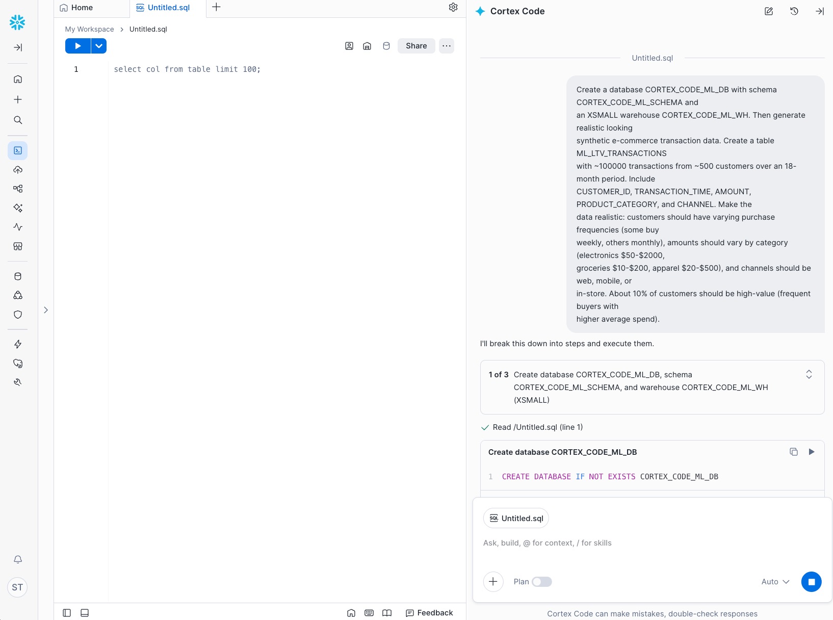
Generate synthetic data by Cortex Code in Snowsight

Cortex Code generates the SQL or Python code to create the database objects and populate the table, then executes it automatically. You will see the code and results appear in a new Notebook cell:

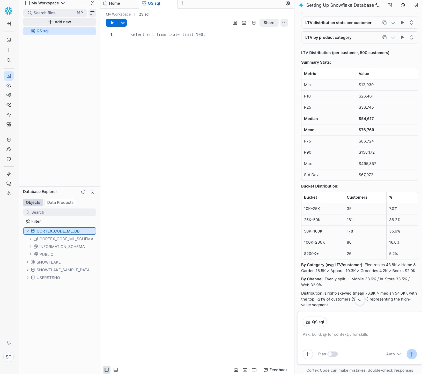
Basic statistics by Cortex Code in Snowsight

Note: Due to the inherent randomness in how LLMs generate text, your results may vary slightly from what is shown in this tutorial.

To verify the data was generated correctly, run the following SQL in a Snowsight worksheet:

Note: COCO_DB.COCO_SCHEMA is an example database and schema. If Cortex Code saved the data to a different database or schema in your environment, update these values before running the query.

SELECT * FROM COCO_DB.COCO_SCHEMA.ML_LTV_TRANSACTIONS LIMIT 10;

You should see 10 rows with columns like CUSTOMER_ID, TRANSACTION_TIME, AMOUNT, PRODUCT_CATEGORY, and CHANNEL.

Alternative: If you prefer to load a pre-built dataset instead of generating data, see Appendix A — Load Pre-Built Dataset from S3 at the end of this guide.

4. Explore the Data (EDA)

Before training a model, analyze patterns to identify the right features for predicting customer lifetime value.

Prompt

Do exploratory data analysis and recommend the features needed to train a regression model that can predict each customer's total spend in the next 90 days.

What Gets Generated

Cortex Code first verifies the table and shows a summary (row count, customer count, date range, and category breakdown), then performs deeper analysis across multiple steps — purchase frequency, spending distributions, recency patterns, and category preferences — and summarizes key findings with recommended features.

If the table is empty (or missing), see Appendix A to load the pre-built dataset and retry.

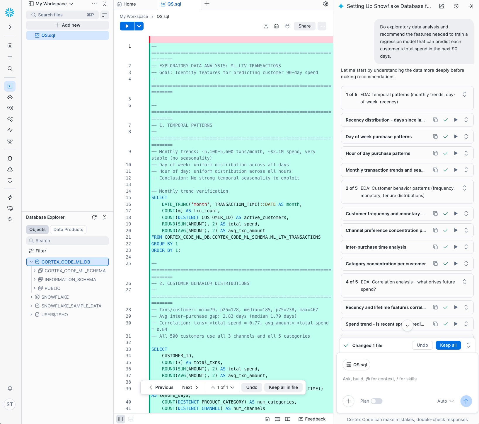
EDA results and feature recommendations in Cortex Code

In this example, Cortex Code identifies signals such as purchase frequency trends, average order value by customer segment, recency of last purchase, and preferred product categories. These insights translate into features like total_transactions, avg_amount, days_since_last_purchase, favorite_category, and channel_distribution.

The EDA step typically reveals patterns such as:

High-value customers purchase more frequently and have higher average order values
Recency of last purchase is a strong predictor of future spend
Certain product categories correlate with higher lifetime value
Channel preferences (web vs. mobile vs. in-store) vary across customer segments

5. Train the Model

With our features identified, we can now train a regression model. XGBoost and Random Forest are excellent choices for this kind of tabular prediction task.

Prompt

Build those features and train a regression model to predict each customer's total spend in the next 90 days. Use two different algorithms, XGBoost and Random Forest, and evaluate the best one. Use 20% of the data as the eval set.

What Gets Generated

Cortex Code typically creates a Notebook, generates feature engineering steps, trains two models, and reports evaluation metrics so you can choose the best performer.

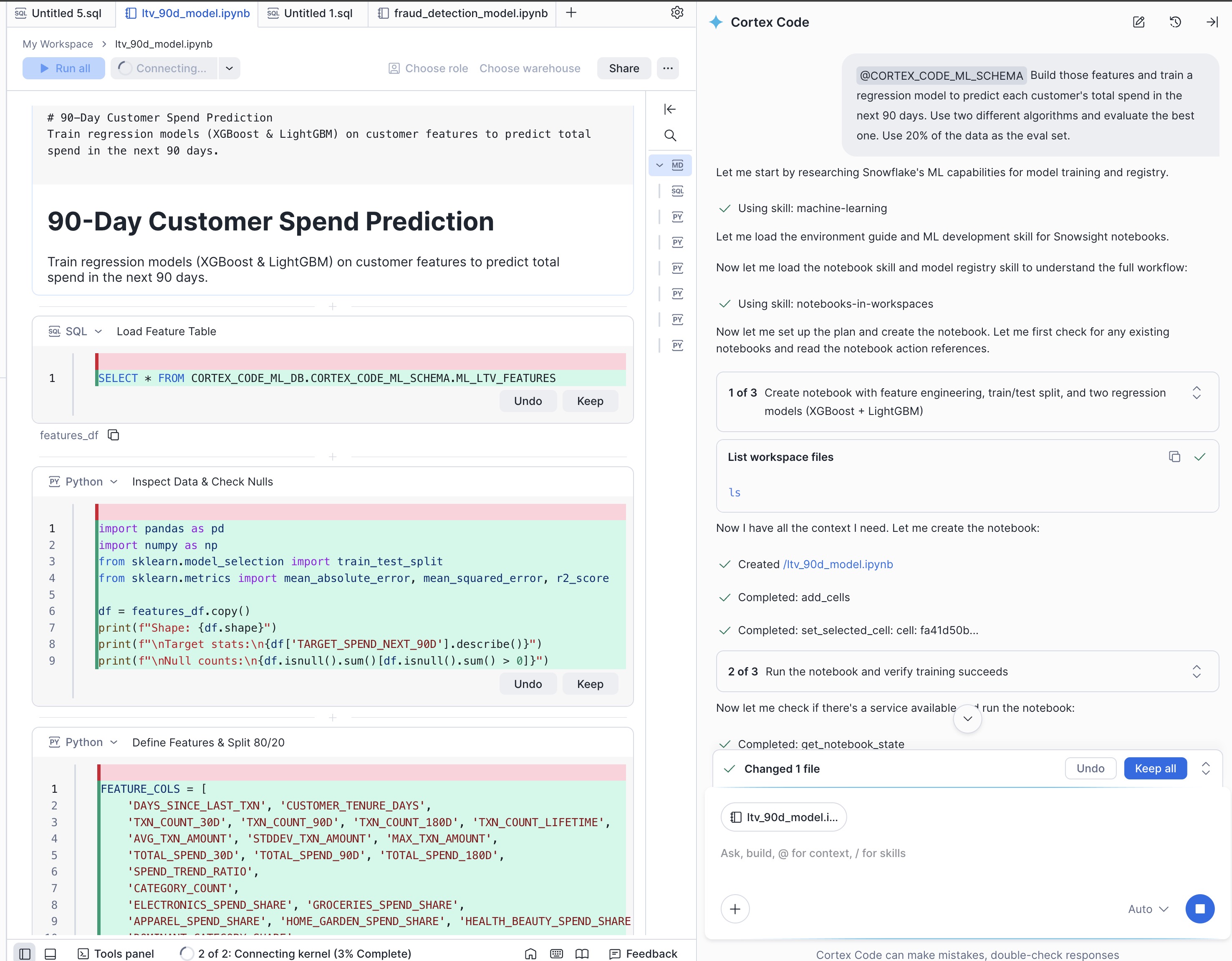
Training and evaluation workflow created by Cortex Code

In this example, Cortex Code generates Python for feature engineering (aggregating per-customer metrics from the transaction history), runs training/evaluation steps, and produces a comparison section (metrics like RMSE, MAE, and R-squared) to help you pick the best model.

Cortex Code will:

Engineer the features based on the EDA recommendations (per-customer aggregations over the training window)
Split the data into training (80%) and evaluation (20%) sets
Train two different regression algorithms (e.g., XGBoost and Random Forest)
Compare their performance using metrics such as RMSE, MAE, and R-squared
Recommend the better-performing model

Review the evaluation metrics to confirm the model meets your requirements before proceeding.

6. Log to Model Registry and Run Inference

Now register the better model to the Snowflake Model Registry and run batch inference.

Prompt

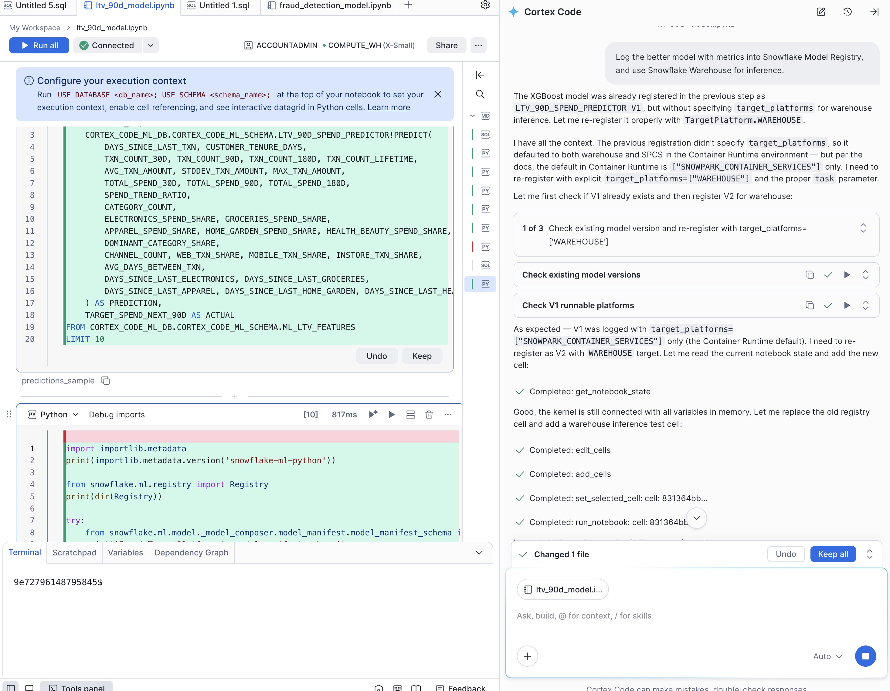
Log the better model with metrics into Snowflake Model Registry, and use Snowflake Warehouse for inference.

Cortex Code handles the log_model() call with appropriate parameters including model metrics, sample input for schema inference, and the target platform set to WAREHOUSE.

Model logged to Snowflake Model Registry with metrics

Then generate predictions:

Prompt

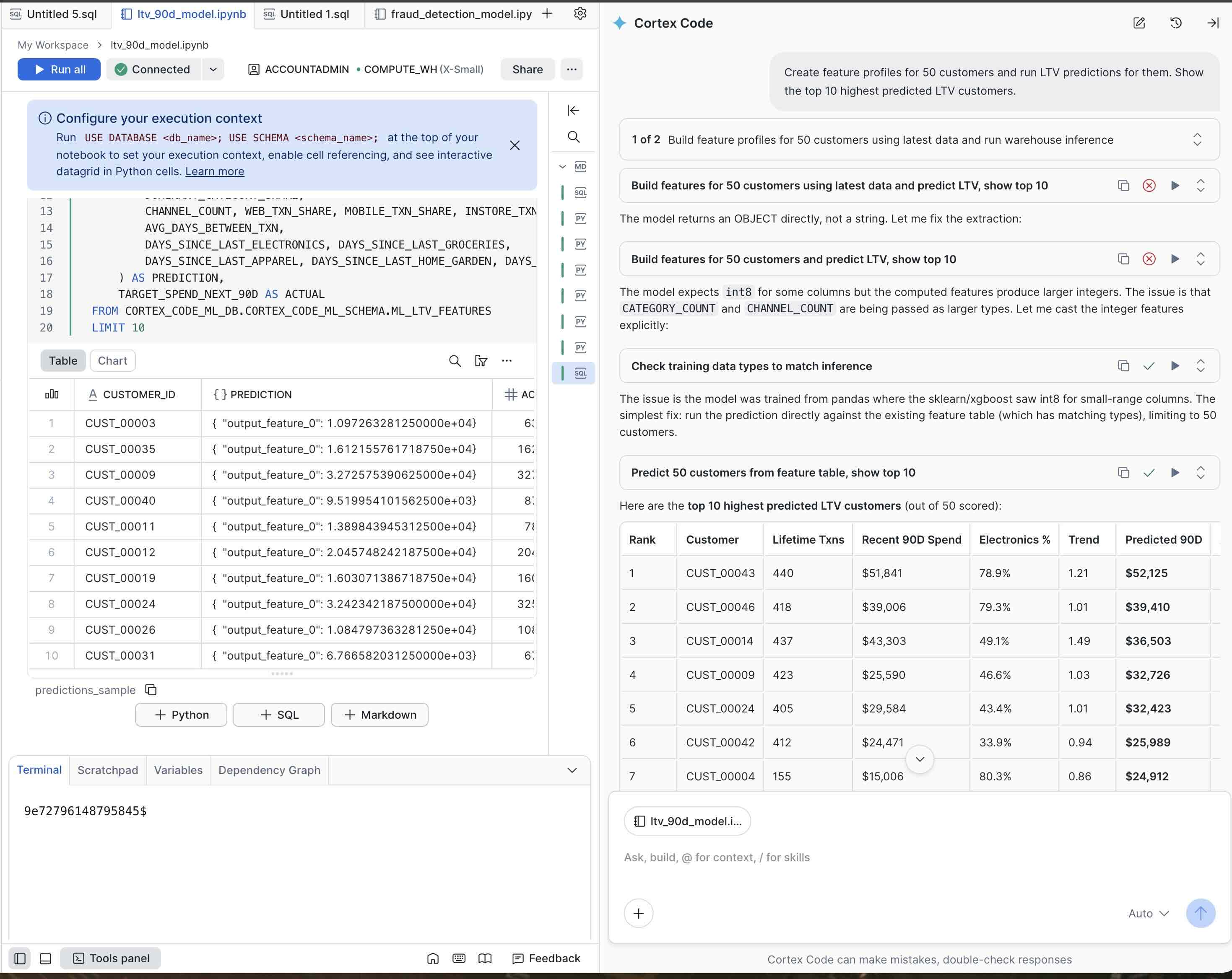
Create feature profiles for 50 customers and run LTV predictions for them. Show the top 10 highest predicted LTV customers.

Cortex Code generates the customer feature profiles, runs inference via your Snowflake Warehouse, and displays the predicted 90-day spend for each customer (sorted by highest predicted LTV).

Batch inference results for LTV predictions

Optional: To deploy the model as a real-time REST endpoint on SPCS instead, see Appendix B — Real-Time Inference on SPCS at the end of this guide.

7. Debug and Recover from Errors

During any natural language coding session, errors are inevitable. The great thing about Cortex Code is its ability to self-correct by assessing the situation, environment, and error to fix issues automatically.

Common Scenarios

Model Registration Errors

When log_model() fails due to parameter issues (e.g., target platform mismatch), Cortex Code diagnoses the error and re-registers the model with corrected parameters automatically.

Notebook Execution Issues

When a cell fails due to missing imports or data type mismatches, Cortex Code detects the issue, adjusts the code, and re-executes the cell.

Feature Engineering Errors

If a feature column is missing or a SQL view fails, Cortex Code investigates the schema, identifies the root cause, and regenerates the feature engineering step.

Best Practices

Start with ACCOUNTADMIN for initial setup, then create dedicated roles
Monitor compute pool resources during SPCS deployment
Review Cortex Code's explanations when it makes corrections
Use the Snowsight Notebook environment for the best interactive experience with visualizations

8. Conclusion And Resources

Congratulations! You've successfully built a complete customer LTV prediction model using only a handful of natural language prompts in Snowflake ML.

What You Built

What You Learned

Generate realistic synthetic e-commerce data with natural language prompts
Perform comprehensive exploratory data analysis with automated feature recommendations
Train and compare multiple regression models for LTV prediction
Log models with metrics to the Snowflake Model Registry
Run batch inference on a Snowflake Warehouse

Related Resources

Web pages:

Snowflake ML - Integrated set of capabilities for development, MLOps and inference leading with agentic ML
Snowflake Notebooks - Jupyter-based notebooks in Snowflake Workspaces
Cortex Code - Snowflake's AI native coding agent that boosts ML productivity

Technical Documentation:

Snowflake ML Documentation - Official Snowflake ML developer guide
Snowflake ML Quickstart - Hands-on guides to get started with Snowflake ML
Cortex Code Documentation - Getting started with Cortex Code
Cortex Code in Snowsight - Browser-based experience
Cortex Code CLI - Command-line experience
Snowflake Model Registry - Register, version, and deploy ML models
Snowpark Container Services - Deploy and manage containerized workloads

Optional A - Cleanup

To avoid ongoing Snowflake credit consumption, you can clean up the resources created in this guide. There are two approaches: a Cortex Code prompt and Manual SQL.

If you completed this quickstart in a single session and your environment does not contain other data, use "A-1 Cortex Code" prompt for a quick cleanup.

If you worked through this quickstart over multiple days or your environment contains resources unrelated to this guide, use "A-2 Manual SQL" approach to ensure you only drop the intended objects.

A-1. Cortex Code

Note: This prompt works best within the same Cortex Code session where the database and other objects like model were created. If you are cleaning up resources from a previous session (e.g., a different day) or your environment contains objects unrelated to this quickstart, use the Manual SQL approach below for more precise control below.

Drop Database and model that we created earlier in this session

Cortex Code will generate and execute the appropriate DROP statements for each resource.

A-2. Manual SQL

If you prefer to run the cleanup manually:

Note: COCO_DB.COCO_SCHEMA is an example database and schema, and COCO_WH is an example warehouse name. If Cortex Code saved the data to a different database or created a different warehouse in your environment, update these values before running the query.

-- Drop the database and all objects within it (table, schema, stage, etc.)
DROP DATABASE IF EXISTS COCO_DB;

-- Drop the model from the Model Registry
DROP MODEL IF EXISTS COCO_DB.COCO_SCHEMA.ML_LTV_PREDICTOR;

-- Drop the warehouse
DROP WAREHOUSE IF EXISTS COCO_WH;

Note: DROP DATABASE removes all schemas, tables, and stages inside it. Make sure you no longer need any of the data before running this command.

Optional B - Cortex Code CLI Walkthrough

The same prompts used throughout this guide work identically in Cortex Code CLI. This section shows CLI-specific setup and sample terminal output so you can compare what to expect in a terminal session.

Setup

Install the CLI:

curl -LsS https://ai.snowflake.com/static/cc-scripts/install.sh | sh

After installing, run cortex and follow the setup wizard to connect to your Snowflake account. For detailed instructions, refer to the Cortex Code CLI documentation.

Verify your connection:

What role am I using and what databases can I access?

Tip: Run Cortex Code CLI inside a VS Code or Cursor terminal to view generated files side-by-side.

Tip: Prefix table names with # (e.g., #COCO_DB.COCO_SCHEMA.ML_LTV_TRANSACTIONS) to ground the conversation to a specific object.

Generate Synthetic Data — CLI Output

After entering the Generate Synthetic Data prompt, Cortex Code CLI shows a summary like this:

  Summary Statistics

  ┌───────────┬──────────┐
  │ Metric    │ Value    │
  ├───────────┼──────────┤
  │ Customers │ 500      │
  ├───────────┼──────────┤
  │ Min LTV   │ $12,930  │
  ├───────────┼──────────┤
  │ P25       │ $36,745  │
  ├───────────┼──────────┤
  │ Median    │ $54,617  │
  ├───────────┼──────────┤
  │ Mean      │ $76,769  │
  ├───────────┼──────────┤
  │ P75       │ $86,724  │
  ├───────────┼──────────┤
  │ Max       │ $495,857 │
  ├───────────┼──────────┤
  │ Std Dev   │ $67,972  │
  └───────────┴──────────┘

  Distribution (Histogram)

    LTV Range           Customers
    $12,930 - $36,868   126  █████████████████████████████████████
    $37,086 - $61,126   170  ██████████████████████████████████████████████████
    $61,382 - $84,439    74  ██████████████████████
    $85,925 - $109,095   35  ██████████
    $110,606 - $133,179  26  ████████
    $134,850 - $157,594  18  █████
    $158,039 - $181,760  19  ██████
    $182,181 - $206,059   7  ██
    $209,265 - $241,987  10  ███
    $257,600 - $283,419   5  █
    $345,815 - $387,939   7  ██
    $410,296 - $495,857   3  █

Explore the Data (EDA) — CLI Output

Cortex Code CLI reads its built-in ML skill, detects the local Python environment, and runs the EDA in incremental steps:

> Do exploratory data analysis and recommend the features needed to train a regression model that can predict each customer's total spend in the next 90 days.

✓  SKILL  machine-learning

✓  READ  cli-environment.md 194 lines

✓  READ  ml-development/SKILL.md 279 lines

* Let me set up the environment and build a comprehensive EDA script.

✓  BASH  which uv
  └─ /Users/shtanaka/.local/bin/uv

✓  BASH  cortex env detect
  └─ {"directory": "/Users/shtanaka/project/sfquickstarts", ...}

✓  BASH  uv venv /Users/shtanaka/project/sfquickstarts/.venv --python 3.10 2>&1
  └─ Creating virtual environment at: .venv

✓  BASH  uv pip install snowflake-ml-python xgboost 

✓  BASH  python session_helper.py  (connectivity check)
  └─ ✅ Connected successfully!

✓  WRITE  /Users/shtanaka/project/sfquickstarts/eda_ltv.py +330

✓  BASH  python eda_ltv.py
  └─ ... (99 more lines)

✓  READ  eda_output/09_feature_importance_rf.png
✓  READ  eda_output/04_correlation_with_target.png
✓  READ  eda_output/01_target_distribution.png

EDA results summary:

  EDA Results and Feature Recommendations

  Dataset Overview
  • 96,264 transactions, 500 customers, 18 months (2024-07-01 to 2025-12-30)
  • Zero nulls across all 5 columns
  • Feature/label split: 80,491 rows for features (before Oct 1, 2025),
    15,773 rows for the 90-day target window

  Key EDA Findings

  Target variable (90-day spend):
  • Right-skewed: median $8,767 vs mean $12,595
  • Range: $1,265 to $85,492

  Correlation analysis reveals two dominant signal families:
  1. Monetary features (r = 0.73–0.93): TOTAL_SPEND, SPEND_90D, STDDEV_TXN_AMOUNT, AVG_TXN_AMOUNT
  2. Frequency features (r = 0.58–0.72): TXN_COUNT, TXN_COUNT_90D, TXN_COUNT_30D

  Random Forest baseline: 5-fold CV R² = 0.646

  Recommended Features — Tier 1 (Strongest Predictors)

  ┌───────────────────┬─────────────┬───────────────┐
  │ Feature           │ Correlation │ RF Importance │
  ├───────────────────┼─────────────┼───────────────┤
  │ TOTAL_SPEND       │ 0.93        │ 0.741         │
  ├───────────────────┼─────────────┼───────────────┤
  │ SPEND_90D         │ 0.88        │ 0.041         │
  ├───────────────────┼─────────────┼───────────────┤
  │ STDDEV_TXN_AMOUNT │ 0.81        │ 0.054         │
  ├───────────────────┼─────────────┼───────────────┤
  │ AVG_TXN_AMOUNT    │ 0.79        │ 0.021         │
  ├───────────────────┼─────────────┼───────────────┤
  │ SPEND_30D         │ 0.78        │ 0.004         │
  └───────────────────┴─────────────┴───────────────┘

Train the Model — CLI Output

> Build those features and train a regression model to predict each customer's
  total spend in the next 90 days. Use two different algorithms, XGBoost and
  Random Forest, and evaluate the best one. Use 20% of the data as the eval set.

✓  READ  experiment-tracking/SKILL.md 456 lines

✓  WRITE  /Users/shtanaka/project/sfquickstarts/train_ltv_model.py +358

* Script details:
  • Features: 28 features from EDA (RFM, spend windows, category/channel shares, trends)
  • Split: 80% train / 20% eval (random_state=42)
  • Model 1 — XGBoost: 500 trees, lr=0.05, early stopping at 30 rounds
  • Model 2 — Random Forest: 500 trees, max_depth=15
  • Experiment tracking: Both runs logged to LTV_90D_SPEND_PREDICTION

✓  BASH  python train_ltv_model.py
  └─ ... training complete

✓  READ  eda_output/10_actual_vs_predicted.png
✓  READ  eda_output/11_residual_distributions.png
✓  READ  eda_output/12_feature_importance_comparison.png

  Model Comparison (20% Eval Set — 100 customers)

  ┌────────┬─────────┬───────────────┬──────────────────────────┐
  │ Metric │ XGBoost │ Random Forest │ Winner                   │
  ├────────┼─────────┼───────────────┼──────────────────────────┤
  │ R²     │ 0.8088  │ 0.7872        │ XGBoost                  │
  ├────────┼─────────┼───────────────┼──────────────────────────┤
  │ RMSE   │ $3,782  │ $3,989        │ XGBoost                  │
  ├────────┼─────────┼───────────────┼──────────────────────────┤
  │ MAE    │ $2,791  │ $2,787        │ Random Forest (marginal) │
  ├────────┼─────────┼───────────────┼──────────────────────────┤
  │ MAPE   │ 37.86%  │ 32.86%        │ Random Forest            │
  └────────┴─────────┴───────────────┴──────────────────────────┘

  Best Model: XGBoost (by R²)

Appendix A — Load Pre-Built Dataset from S3

If you prefer to load a pre-built dataset instead of generating synthetic data with Cortex Code, run the following SQL in a Snowsight SQL Worksheet or paste it as a prompt in Cortex Code CLI. You can also download setup.sql.

USE ROLE ACCOUNTADMIN;

CREATE DATABASE IF NOT EXISTS COCO_DB;
CREATE SCHEMA IF NOT EXISTS COCO_DB.COCO_SCHEMA;
CREATE WAREHOUSE IF NOT EXISTS COCO_WH
  WAREHOUSE_SIZE = 'XSMALL'
  AUTO_SUSPEND = 60
  AUTO_RESUME = TRUE;

USE DATABASE COCO_DB;
USE SCHEMA COCO_SCHEMA;
USE WAREHOUSE COCO_WH;

CREATE OR REPLACE FILE FORMAT ml_csvformat
  SKIP_HEADER = 1
  FIELD_OPTIONALLY_ENCLOSED_BY = '"'
  TYPE = 'CSV';

CREATE OR REPLACE STAGE ml_ltv_data_stage
  FILE_FORMAT = ml_csvformat
  URL = 's3://sfquickstarts/sfguide_getting_started_with_cortex_code_for_ds_ml/ltv_transactions/';

CREATE OR REPLACE TABLE ML_LTV_TRANSACTIONS (
	CUSTOMER_ID VARCHAR(16777216),
	TRANSACTION_TIME TIMESTAMP_NTZ(9),
	AMOUNT NUMBER(12,2),
	PRODUCT_CATEGORY VARCHAR(15),
	CHANNEL VARCHAR(8)
);

COPY INTO ML_LTV_TRANSACTIONS
  FROM @ml_ltv_data_stage;

SELECT 'Setup complete — ML_LTV_TRANSACTIONS loaded.' AS STATUS;

After running the SQL, return to the Explore the Data step.

Appendix B — Real-Time Inference on SPCS

As an alternative to batch inference on a Snowflake Warehouse, you can deploy the model as a REST endpoint on Snowpark Container Services (SPCS) for real-time inference.

Prerequisite: A compute pool configured for Snowpark Container Services.

Prompt

Log the better model with metrics into Snowflake Model Registry, and use SPCS to create a REST endpoint for online inference.

Cortex Code handles the log_model() call with the target platform set to SNOWPARK_CONTAINER_SERVICES, then creates the SPCS service and endpoint for real-time inference.

Then test the endpoint with latency profiling:

Prompt

Create feature profiles for 50 customers and run LTV predictions using the REST API for online inference running on SPCS. Show the top 10 highest predicted LTV customers and a latency profile (p50, p95, p99).

Cortex Code sends HTTP requests to the SPCS REST endpoint and displays results including:

Predicted 90-day spend for each customer profile
Per-request latency measurements
A latency profile summary (p50, p95, p99) to help you understand the real-time performance characteristics of your deployment

Updated 2026-05-07

This content is provided as is, and is not maintained on an ongoing basis. It may be out of date with current Snowflake instances