Routing Inside Snowflake, Part 2: Precomputing Travel-Time Matrices with H3

Part 2 of a two-part series. In Part 1, we made the buy-vs-build case for running routing inside Snowflake and walked through the cost and governance picture.

TL;DR

For routing workloads that only ever read travel time and distance — dispatch, ETAs, reachability, batch backtests — you don't need a live routing engine at all. Precompute the answers once into an H3-tessellated travel-time matrix, store it in a Snowflake table, and serve it as a SQL lookup with no compute pool warming needed.

When is the live engine more compute than you need?

Both of the "Build" costs we covered in the first part — the build cost and the serving cost — assume the routing engine is the thing answering every routing question. For some workloads, that is more compute than the question requires. The live engine pays the same compute cost whether the caller wants a turn-by-turn route or only the travel time and distance, and the Snowpark Container Services pool kept warm to answer those questions pays for the polyline work whether or not anyone consumes it.

For fleets running high-frequency ETAs, dispatch decisions, or batch arrival-time backtests — workloads where the route shape itself is never read — there is a cheaper architecture, and DoorDash described it publicly in its 2025 "How DoorDash achieves fast travel estimates" engineering post: rather than ask the engine the same travel-time question over and over, precompute the answers once, store them as data, and look them up at query time. DoorDash runs the open source OSRM engine inside a Spark cluster and persists the results to Redis.

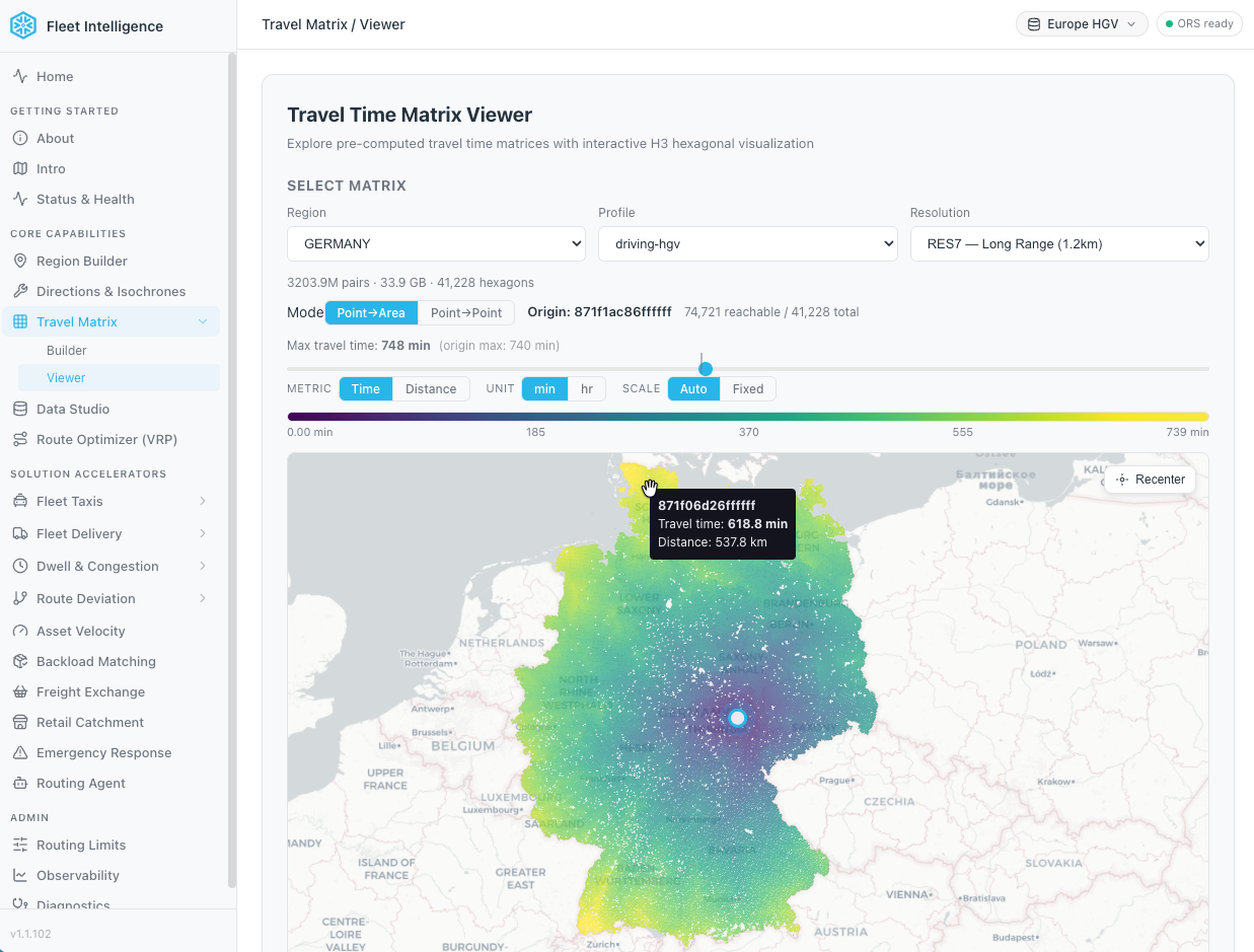
How the precomputed travel-time matrix works

The operating area is tessellated into H3 hexagons — Uber's open source hierarchical hexagonal grid — and the routing engine is asked to compute the travel time and distance between every pair of cells. The result is one Snowflake table per region per profile per resolution, keyed by origin hexagon and destination hexagon, with travel time and distance as the payload — built once and reused for every subsequent query.

At query time, the matrix is a table: a SQL lookup against the clustered hexagon-pair returns travel time and distance in milliseconds against a warehouse — no compute pool active, no engine warm-up. A fleet that previously kept a runtime pool warm to answer every ETA can serve the same workload from the materialized table instead, calling the live Routing engine only for the queries that need a polyline.

You can explore precomputed travel-time matrices for the UK, Germany and California available on Snowflake Marketplace and published by Dekart.xyz.

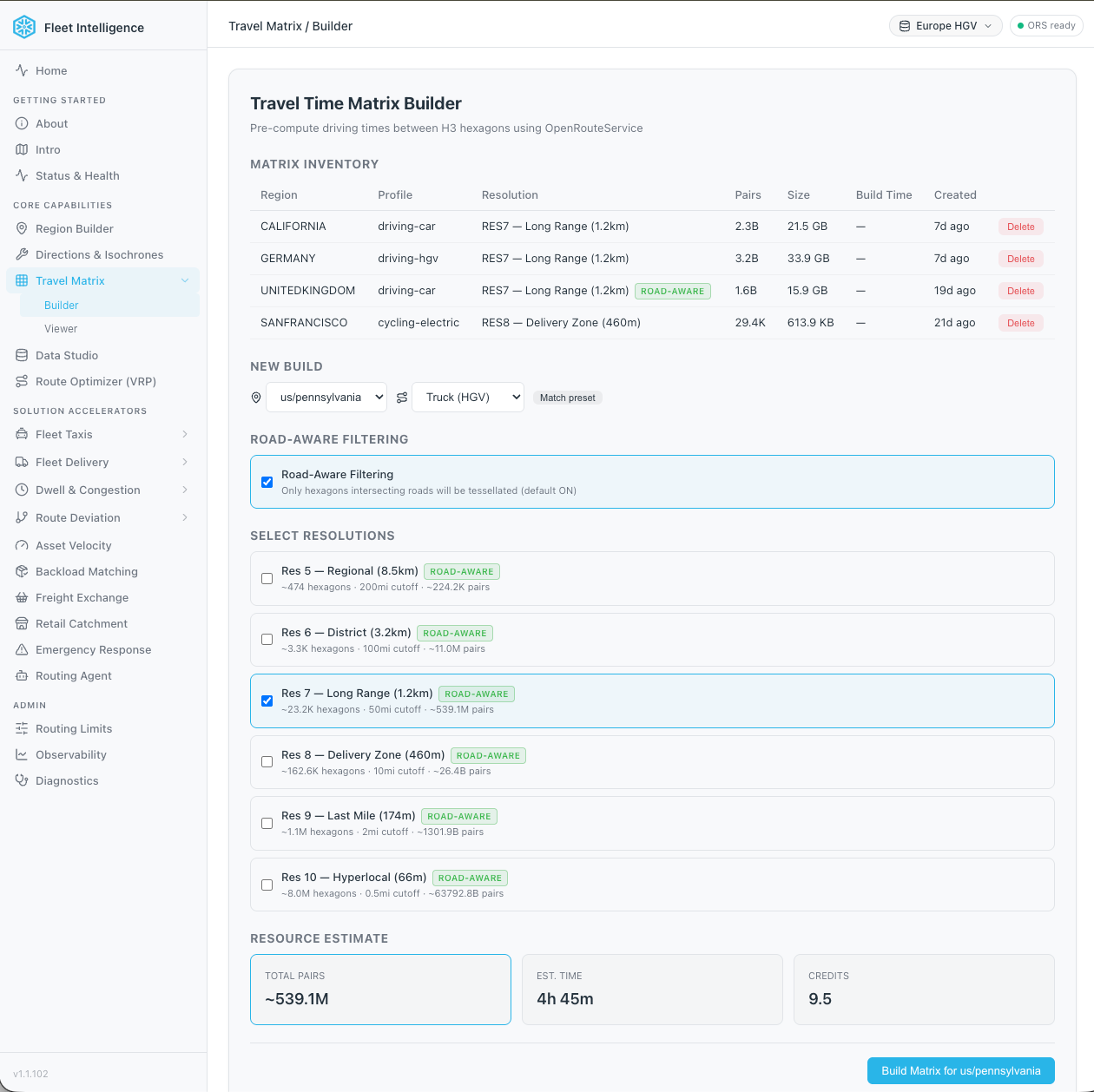
Road-aware tessellation

Tessellating the bounding box directly enumerates every hexagon inside it, including the ones over water, mountains or other terrain with no roads. For a city, those empty hexagons are a small fraction of the total. But a bounding box around the United States contains hexagons over mountain ranges, deserts and other areas with no road network, and because the matrix scales quadratically with hexagon count, every empty hexagon shows up both as an origin and as a destination — paying twice over for routes that lead nowhere useful.

We address this with a step that runs before the matrix build itself: a spatial semi-join in SQL against the Overture Maps Transportation dataset — available as a Snowflake Marketplace listing — that keeps only the hexagons containing at least one road segment. Hexagons over open water, wilderness or other roadless terrain are dropped before the matrix job sees them. For a region the shape of San Francisco, where roughly 40% of the bounding box is ocean, the hexagon count drops by up to 40% and the API call count drops by around twofold. For a country-sized region with significant water, mountains, or empty terrain, the reduction is larger.

Tradeoffs of the H3-based travel-time matrix

The H3-based pattern carries three tradeoffs.

Granularity is bounded by hexagon size. Smaller cells mean more precise answers but a quadratically larger matrix to build, since every cell pairs with every other cell, bigger cells are cheaper to build but answer with more error, and short trips can collapse into the same origin-destination cell, where the matrix returns zero distance. DoorDash addresses this by storing each location at three H3 resolutions side-by-side and selecting the highest available resolution at query time. The same is achievable here — the matrix builder accepts a resolution argument, so an operator can build matrices at multiple resolutions for the same region.

The matrix only answers travel-time and distance questions, not route shape. Applications that need the actual route — turn-by-turn navigation, deviation analytics, route visualization — still call the live Route Service engine for those.

The matrix is only as fresh as the last build. Map updates, weight changes or new profiles require a rebuild. For routing graphs that are themselves rebuilt monthly or quarterly, that is consistent with their cadence; for workloads where this morning's road closure must be reflected in this afternoon's ETAs, the matrix is not a fit.

Which table shape should you use for the matrix?

Once the precomputed matrix exists, the question is how to serve it. A matrix is just a Snowflake table, but Snowflake offers several table shapes, and routing applications hit them with two very different patterns:

• Operational queries — a dispatcher matching one driver to one destination, an ETA API answering "how long from A to B?" — are point lookups.
• Analytical and visual queries — for example, a reachability map shading everywhere a vehicle can get to in 30 minutes, an isochrone overlay or any other use case that requires reading all destinations reachable from one origin — can be thousands of rows.

We benchmarked four variants on the same Heavy Goods Vehicle (HGV) transportation type in Germany and H3 resolution 6 (a travel-time matrix table with 121 million rows) — Standard, Standard with Clustering, Hybrid (Unistore) and Interactive — serially and under a concurrency sweep at 1, 10, 50 and 100 workers.

Hybrid (Unistore) excels on point lookups and easily holds 400 QPS at one hundred workers with p95 not exceeding 350 ms. For group lookups Interactive led at every concurrency level.

The fit is therefore pattern- and duty-cycle-specific:

• High-concurrency point lookups (dispatch APIs, near-real-time ETA updates) — Hybrid (Unistore).
• Always-on reachability surfaces (isochrones, dashboards in continuous use) — Interactive tables.
• Intermittent analyst queries and periodic batch jobs — clustered Standard table.

The precomputed matrix is just a table — which kind sets whether the bill scales with traffic or with wall-clock time.

Leveraging the Routing Engine from specialized spatial analytics tools

The SQL functions exposed by the Routing Engine are the powerful primitives to enable scalable routing processes within Snowflake, but, to wire them into production workflows some analytics teams would like to call them from their cloud-native GIS platform of choice.

In this regard, CARTO's recent Workflows Extension Package for Snowflake ORS already provides this level of integration. Each routing function — Directions, Isochrones, Matrix and Optimization — is wrapped as a drag-and-drop component in CARTO Workflows, composable into parameterized pipelines that analysts and data scientists can build, share, schedule and rerun without writing SQL. Every pipeline pushes down calls to Snowflake, so there is no API key juggling and no movement of data out of the governance perimeter.

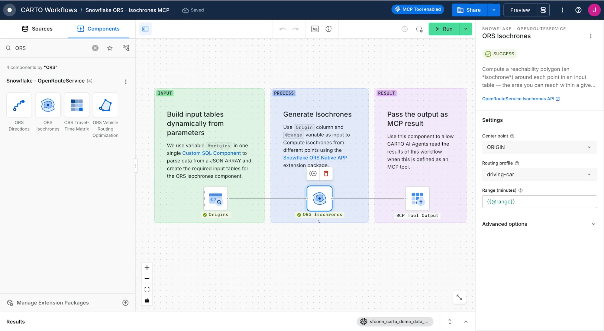
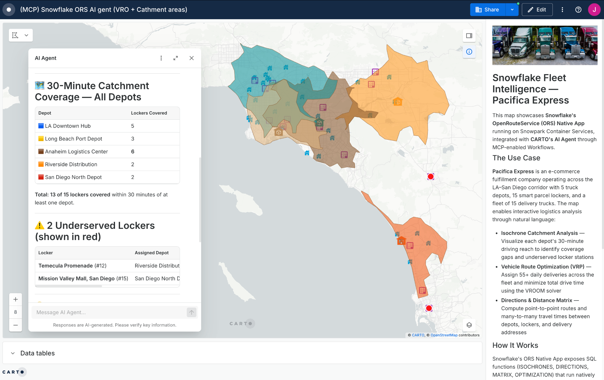
What changes when those pipelines are exposed to AI agents is the ceiling on throughput. Any parameterized CARTO Workflow can also be published as an MCP tool through the CARTO MCP Server. The same routing pipeline an analyst composes in CARTO becomes a deterministic tool an AI agent can call autonomously. Additionally, CARTO's CLI and MCP Server make the platform fully compatible with Cortex Code and Snowflake CoWork, enabling users to create workflows, maps and geospatial agents in CARTO without leaving Cortex Code's interface and giving business teams access to geospatial analysis procedures as MCP tools on Snowflake CoWork.

Key takeaways

• Precomputed travel-time matrices turn routing into a SQL lookup: For workloads that only need travel time and distance, an H3-tessellated matrix eliminates the need for a live engine entirely.
• Road-aware tessellation cuts the build: A spatial semi-join against Overture Maps drops roadless hexagons before the matrix job runs, and because the matrix scales quadratically, the savings compound.
• Table shape matters: Hybrid (Unistore) wins on high-concurrency point lookups, Interactive wins on group reads, Standard wins on intermittent batch workloads.
• Match freshness to cadence: The matrix is as fresh as its last build — ideal for monthly/quarterly graph cadences, not for same-day road closures.

Missed the cost and governance case? Read Part 1: Running Routing Inside Snowflake — From Per-Call to Per-Compute. If you want to try a self-hosted routing service for one of your use cases, use this skill in CoCo CLI and after about 30 minutes of unattended installation, you'll see a freshly baked routing service in your Snowflake account. Test it out today and let us know what you think!