

Every Snowflake Standard warehouse you run operates as an independent pool of compute, separate from your other warehouses. Queries routed to it can draw on its available capacity, while queries routed elsewhere cannot. This isolation provides per-workload cost controls, service-level agreements (SLAs) and accounting — but it also means that idle capacity on one warehouse cannot relieve a queue building on another.
The question is whether you can keep the boundaries without the waste. This post works through how Adaptive Compute does it: shared compute, per-query sizing, two properties that replace 15 and the admission control underneath.
This is the first in a series on Adaptive Compute.
Four principles
Adaptive Compute is built around four principles. Each one addresses a place where the Standard warehouse model asks you to make a decision in advance that the platform is better positioned to make in the moment.
Shared compute: Many workloads draw from one pool instead of each warehouse holding its own idle capacity. Idle time in one workload is spent running another's queries rather than sitting reserved and unused.
Autosizing: Every query runs at the size that fits it, rather than a single size chosen in advance and applied to all of them.
The latest hardware and software acceleration: You stay on the newest hardware and query-acceleration techniques automatically; no action needed to upgrade or reconfigure.
Ease of use: A Standard warehouse exposes over 15 properties to get right; Adaptive collapses that into two. Warehouse sizes, multi-cluster settings, Query Acceleration Service configuration, and suspend and resume policies all stop being yours to manage.
Shared compute
Adaptive works by changing what sits underneath your warehouses. Every job across every Adaptive warehouse in an account is routed to a pool of compute dedicated to that account — never shared with other accounts, and never with other warehouse types. Your warehouses remain distinct endpoints for organizing, governing and reporting on workloads; the compute that runs the queries is pooled beneath them.
To see why that matters, stop looking at any one warehouse and zoom out to the compute your account uses as a whole. What you find is not a pool: it is many isolated islands of compute, one per running warehouse, each sized and billed on its own. Capacity inside an island is reachable only by queries routed to that particular warehouse. Nothing else in the account can use it, however much it is needed elsewhere.
This is structural. Once compute is partitioned by warehouse, each has to be provisioned for its own peak, and every peak not currently happening is capacity nobody can use.
There are three main ways we see customers organize compute across all those warehouses, and until Adaptive you had access to the first two:
Isolated warehouses: Each one reserves idle headroom it never uses, so the consolidation savings are never realized.
A few large, consolidated warehouses: This reclaims the idle time, but it complicates query routing and dissolves the per-workload boundaries that cost controls and SLAs depend on.
Shared compute: Delivers the consolidation savings and keeps those per-workload boundaries intact.
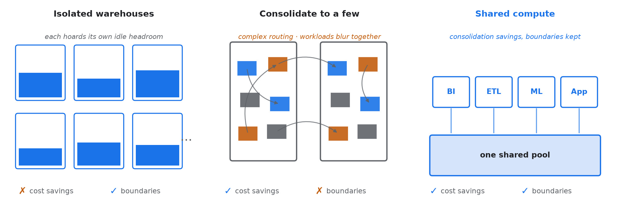
Figure 1: Isolated warehouses lose consolidation savings. Consolidated warehouses lose per-workload boundaries. Shared compute is the only column with a check in both rows.
There is a compounding benefit worth noticing. The more warehouses you move to Adaptive, the larger the pool's aggregate demand, and the more opportunity the system has to place queries efficiently. The economy of scale works in your favor — which is also why moving a single warehouse in isolation shows the least benefit.
Autosizing: each query gets its own size
A classic warehouse forces a single size for every query — too much for the small ones, not enough for the large ones. Adaptive manages a distribution instead, placing each query at its own size.
Almost no real workload is uniform. The same warehouse might serve a dashboard refresh that scans a handful of partitions and a nightly transform that joins billions of rows. A Standard warehouse asks you to settle that in advance with one setting, and whichever size you pick, both ends pay for it. An Adaptive warehouse decides per query, on the evidence of the query itself, so the compute it hands out follows the shape of the demand rather than a number chosen ahead of time.
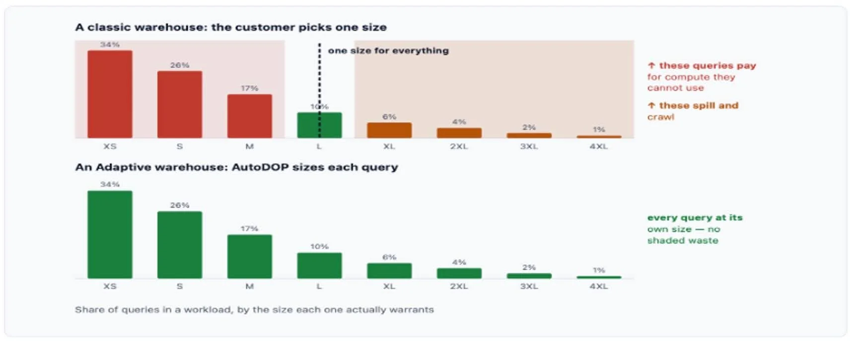
Figure 2: The bars show the same workload — the share of queries that warrant each size. Top: a fixed-size warehouse draws one line through the distribution; everything left of it overpays, everything right of it is undersized. Bottom: an Adaptive warehouse runs each query at the size it warrants.
The efficiency payoff
That per-query decision is where the efficiency comes from. Small queries stop consuming compute they cannot use. The capacity saved here funds the headroom for your heavy queries. It also allows the same spend to handle more work.
Faster is not free
But faster is not free. Each query has its own performance curve: speed climbs as compute is added, then flattens into a scaling wall beyond which additional compute yields little additional speed.
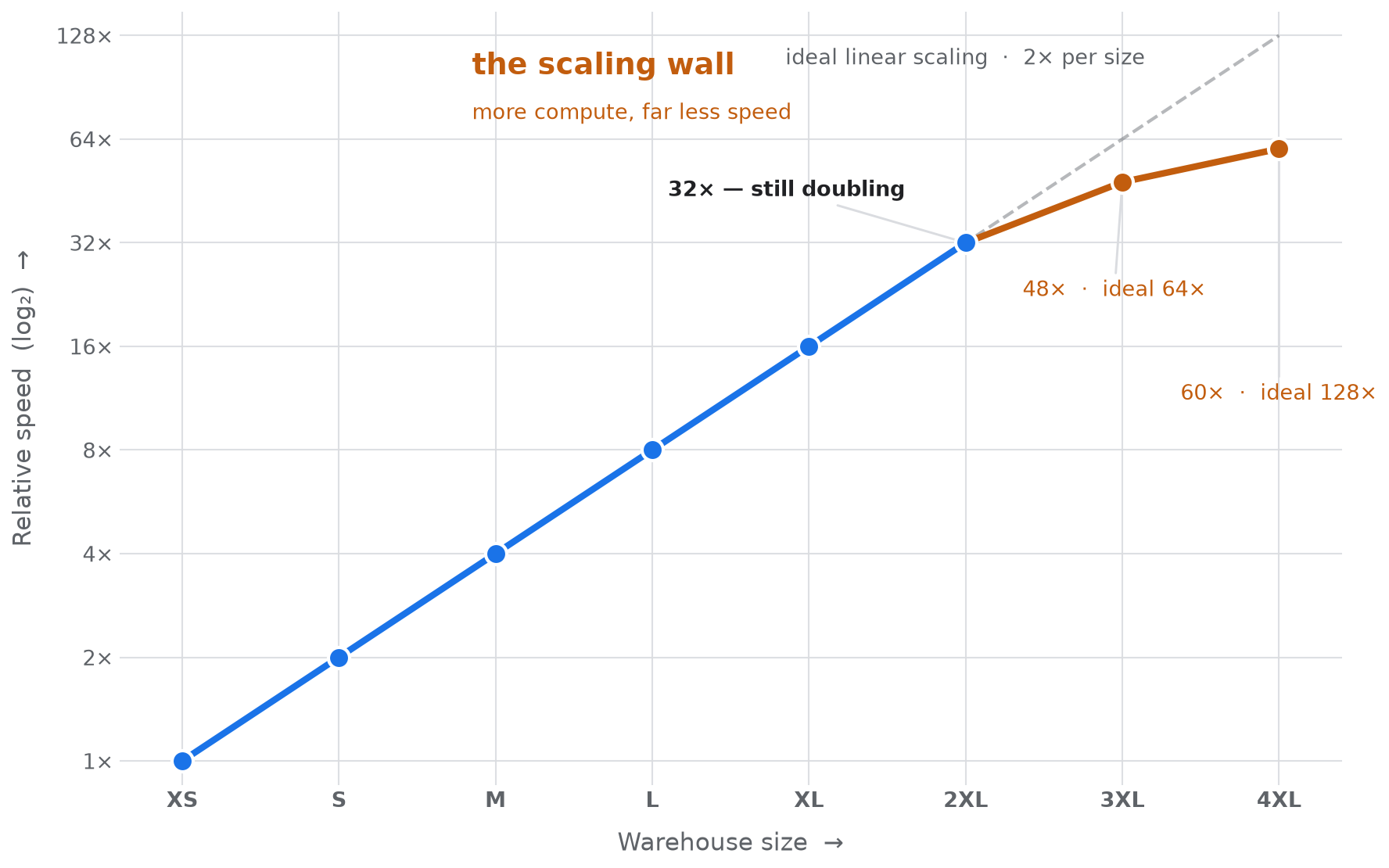
Figure 3: One query's speed at each warehouse size. It scales almost ideally up to 2XL — each size doubling speed — then hits a wall. The jump from 2XL to 3XL doubles the compute but buys only 50% more speed instead of 100%. From 3XL to 4XL, another doubling of compute for just 25% more speed. There is no single "right" size: there is a price-performance curve, and every workload wants to opt out at a different point on it. Deciding where to opt out is what tuning an Adaptive warehouse comes down to.
Snowflake predicts this curve before the query runs. At compile time it already knows the data volume, the join structure and how much of the work can proceed in parallel — enough to estimate speed and cost at every size the query could run on.
So the system knows the cost-performance trade-offs. What it cannot know is which trade-offs you are willing to make. A 2x increase in compute that buys 1.5x the speed may be a bad deal for a background batch job and a perfectly reasonable one for a report someone is waiting on. The same point on the same curve is worth it or not depending on the workload — and that is a judgment about your business, not a fact about the query.
That gap — between what the system can measure and what only you can decide — is why the two Adaptive Compute properties exist. MAX_QUERY_PERFORMANCE_LEVEL (MQPL) records how far up the cost-performance curve a single query is allowed to go — how much speed is worth paying for. QUERY_THROUGHPUT_MULTIPLIER (QTM) records how much concurrent work the warehouse should admit before new queries queue — how much of a burst is worth absorbing. Together, they let the system enforce your cost-performance trade-off on every query, without you having to intervene one query at a time.
The three questions to answer about your business
Where you opt out on the curve is a business call. Three questions locate it, and all three are about your business rather than your data:
- How much does latency actually matter for this workload, and to whom? Is someone waiting in front of a dashboard, is a critical report at risk of missing the start of the business day, or is it an overnight batch job that only has to finish by morning? That sets how aggressively your typical query trades money for speed.
- How far am I willing to let an unusually demanding query go? Your heaviest queries can justify far more compute than your typical ones, and that headroom is worth having — up to the point where the bill for a single query becomes unacceptable.
- How do bursts impact my business? Does a surge of requests queue until users lose interest, or does it simply mean a nightly report takes a little longer while still finishing on time? What one query may spend says nothing about 50 of them arriving together.
Answer these three and you have stated your policy. Two properties record the answers — the first covers questions one and two, the second covers question three.
MAX_QUERY_PERFORMANCE_LEVEL (MQPL)
MQPL answers questions 1 and 2 — the ceiling on how far up its curve any single query may climb.
A good starting point is one size above your old Standard size. Your classic size is the performance envelope your everyday queries already live in (question 1), and the extra size is headroom for the occasional heavy query that can put it to use (question 2). Setting MQPL equal to your classic size means giving up that headroom for outliers and accepting a lower baseline for everyday performance than you were accustomed to on Standard.
What it does. MQPL is a ceiling — it binds absolutely. Even when the next step up on a query's curve is a good deal — real speed for a modest amount of extra cost — MQPL says no further. A good deal is still a bigger bill, and you have already told the system where you are willing to stop.
What it isn't. It is not an instruction to run at that level, and it is not a warehouse size. On a Standard warehouse the size is what every query runs at; on an Adaptive warehouse MQPL is the maximum any single query may reach. Most queries land below it, sized on what each can actually use. The ceiling only trims the top.
MQPL is expressed in the familiar t-shirt sizes, XS through 4XL. Once set, it generally does not need revisiting: it states a preference about a trade-off, not a snapshot of today's workload.
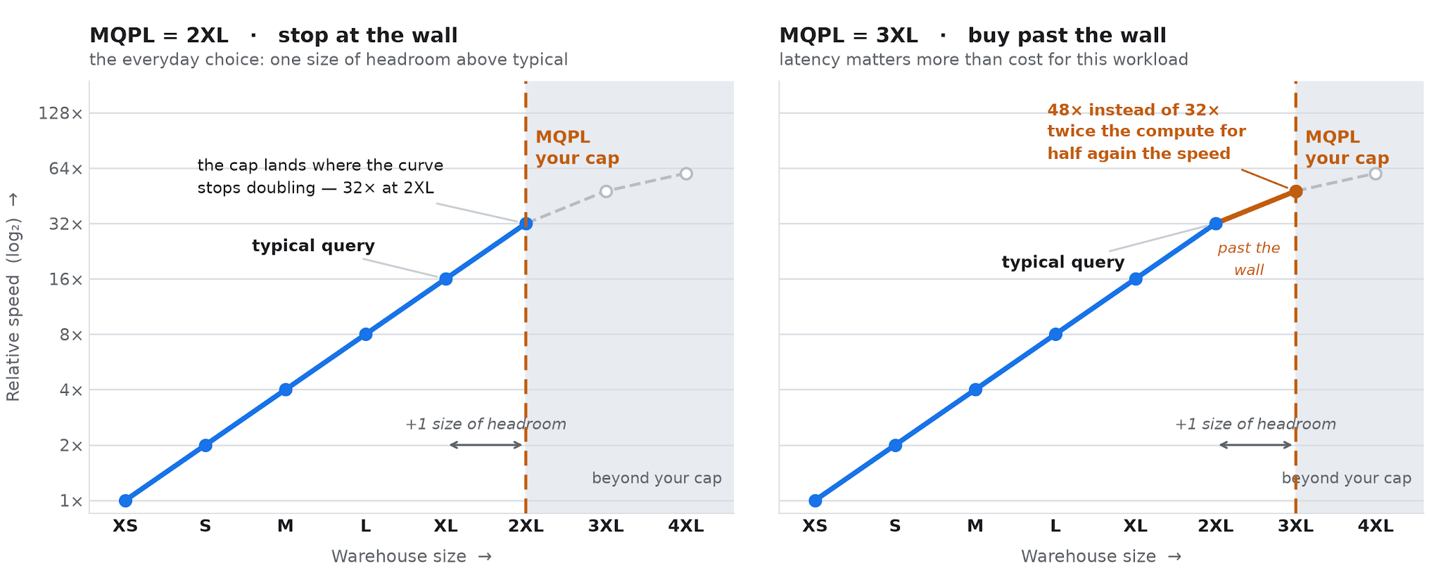
Figure 4: The same curve, two different caps. The typical query marker is the size your everyday queries settle at; MQPL is the ceiling one size above it.
On the left, typical is an XL and the cap lands at 2XL — right where this query stops doubling, so nothing is allowed past the wall.
On the right the everyday queries are heavier and already run at 2XL, so the same one size of headroom puts the cap at 3XL: past the wall, paying twice the compute for half again the speed. Same rule, different landing point. Neither is the correct answer — the right is what you accept when latency matters more to the business than the marginal cost of getting there.
Where you stop is a business decision. The scaling wall is not a rule about where MQPL belongs. For most workloads, stopping at or near it is the sensible default. Some workloads are worth it anyway — a report with a hard deadline, a query on the critical path for everything downstream. MQPL is where you record that judgment.
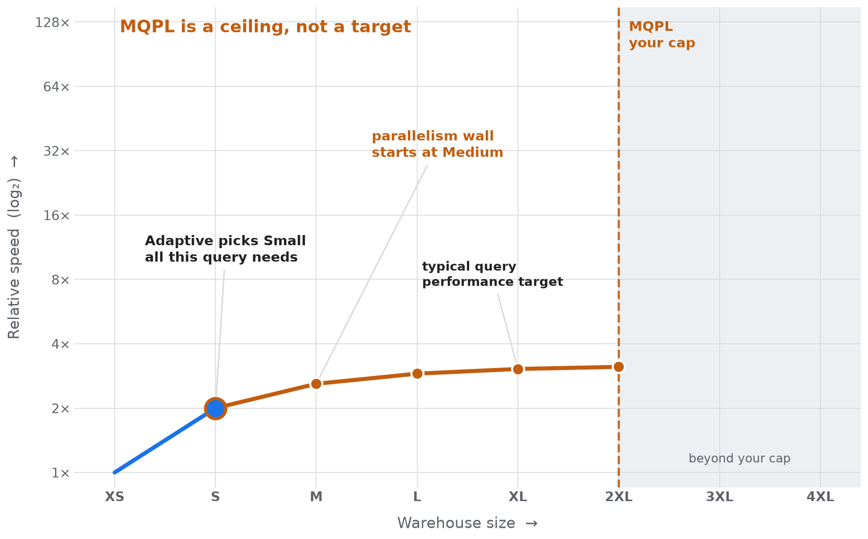
Figure 5: MQPL is a ceiling, not a hard target. Same cap as the left panel of Figure 4 (2XL) — but this query's parallelism wall starts at Medium, so past Small it barely speeds up. Adaptive gives it only Small, the size it can actually use, and the 2XL ceiling never comes into play. You set the ceiling; each query's own wall decides its size — so you never use compute that you can't turn into speed.
When Adaptive does not have a confident read on a query — an unfamiliar shape, a new plan, not enough history — the policy is to do no harm rather than guess: the query runs at the level it would have been given before. A second guardrail keeps a floor under how far down it will size. Both are safeguards against today's uncertainty rather than permanent parts of the design.
QUERY_THROUGHPUT_MULTIPLIER (QTM)
QUERY_THROUGHPUT_MULTIPLIER (QTM) answers question 3 — it scales how much concurrent work the warehouse admits before queries wait in a queue. It is a multiplier, not a query count: the concurrency it buys is relative to your MQPL.
Workloads rarely arrive at a steady rate. The dashboards all refresh at 9 a.m. A pipeline fires 40 transforms in parallel. A concert goes on sale and the requests land in the same few minutes.
QTM tells Adaptive how much of that surge to take on at once, rather than holding part of it back in a queue. That queue is not just a limit — it is a control. Letting some queries wait is how the business applies back pressure: rather than scaling out without bound and paying for every burst at its peak, you decide how much a surge is worth.
- Raise QTM and more runs at once → lower latency, higher peak cost
- Lower QTM and queries queue → slower under load, but spend stays capped.
Queueing is the lever that trades latency for cost, and QTM is where you set it. It is expressed as a multiplier of your chosen MQPL, so the default already reflects the performance level you asked for. And much like MAX_CLUSTER_COUNT on a Standard warehouse, it provides headroom to absorb spikes rather than a fixed allocation: if your workload doesn't burst into that additional capacity, setting it higher won't affect your bill. If a burst does use it, your bill may increase accordingly.
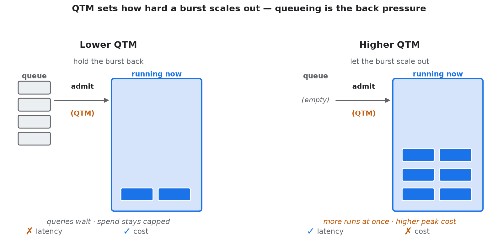
Figure 6: QTM tunes queueing. A lower QTM holds a burst back — queries wait, so peak spend stays capped. A higher QTM lets the burst scale out — more runs at once, at a higher peak cost. Neither is strictly better; which you want is a business call, and queueing is how you enforce it.
Together, MQPL and QTM replace the dozen-plus properties a Standard warehouse requires you to manage — one dial for single-query performance, one for throughput and the cost of bursts.
Under the hood: admission control
MQPL and QTM are not just tuning dials. Together they define an admission-control token budget, and every query passes through admission control before it runs against the shared pool. That token budget is what admission control uses to decide which queries run now and which wait.
The mechanism is straightforward. MQPL and QTM combine into an admission-control budget for the warehouse, expressed as a supply of tokens. How they combine is where QTM gets its name: it is a multiplier on MQPL, issuing tokens in multiples of the performance level you chose. Loosely, this provides enough tokens to run the number of concurrent queries that QTM is currently configured to, where each query running at the full MQPL size — if MQPL is Large and QTM is 4, the warehouse can concurrently execute the equivalent of 4 concurrent Large queries worth of compute. One property sets how big a query may get; the other sets how many of those you can afford at the same time. The product of the two is the admission-control token budget.
That admission-control token budget represents the warehouse's available execution capacity. During compilation, each query is assigned an abstract token requirement based on the resources it needs. A query begins running when enough capacity is available; those tokens are reserved while it runs and returned when it completes. If insufficient capacity is available, incoming queries wait until capacity is released.
Sharing compute also changes a query's token cost, which reflects the compute unit it is actually assigned to rather than a flat per-query rate: a query with a unit to itself carries the whole unit, while a query sharing one carries only its fraction. Because shared queries tie up fewer tokens each, more of them can be admitted at once.
Tokens are fungible
Tokens make the budget fungible. It is not four fixed Large-shaped slots — it is a pool the system can spend in whatever combination fits the workload: four Large queries, eight Medium, 16 Small or any mix within the budget. That is why a workload with a wide spread of query sizes thrives on a single Adaptive warehouse.
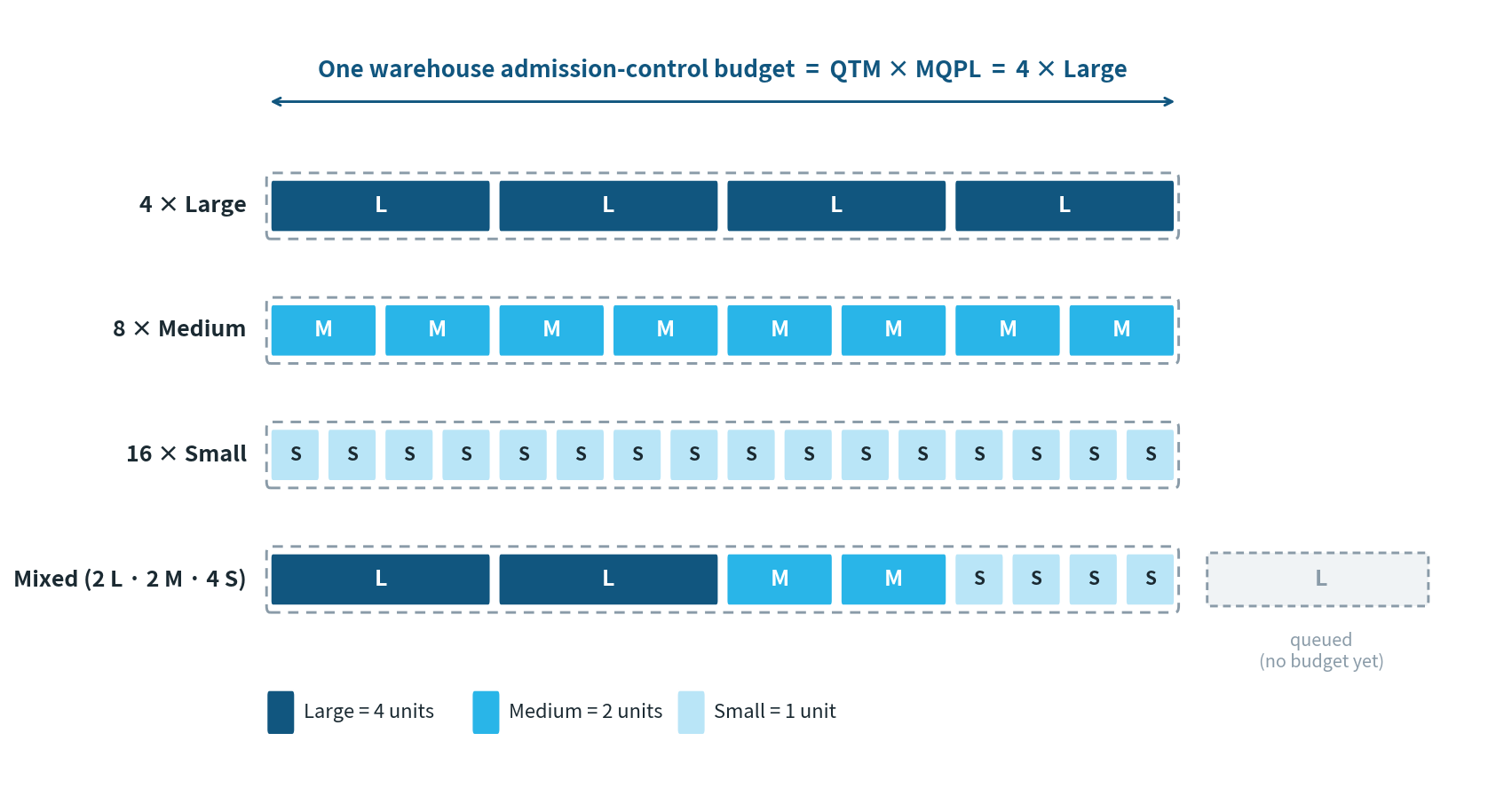
Figure 7: One budget, many shapes. The same QTM × MQPL budget can fund four Large queries, eight Medium, 16 Small or any mix that fits. Queries that do not fit wait until running queries return their tokens.
The bottom line
Standard warehouses fragment compute into isolated islands and force workloads with diverse query needs into a single size, turning price-performance into an administration problem that has to be resolved every time the workload evolves. Splitting a workload across several warehouses by query size recovers some of that efficiency, but it sacrifices the ability to report and govern on business purpose.
Adaptive delivers the efficiency without the fragmentation: a shared compute model that matches each query to the resources it can actually use, a full distribution of sizes within a single warehouse, and cost and telemetry still anchored to the workload. You stop sizing infrastructure and start defining workloads. Snowflake handles the rest.