Oct 1, 2026/9 min readMachine Learning
Operationalizing Model Serving: Completing the Feedback Loop with Snowflake


Deploying machine learning (ML) models is the start of the journey, not the end. Organizations frequently allocate significant resources to model development, only to encounter restricted visibility once models enter production systems. Inference data is often fragmented across disparate logging mechanisms, while active model versions remain unindexed at the point of prediction. This systemic lack of transparency impedes rigorous root-cause analysis and escalates operational risk during model deployment cycles.
Snowflake ML’s inference infrastructure is designed to resolve this architectural disconnect. From initial registration within the Model Registry to execution on Snowpark Container Services (SPCS), the platform automatically captures prediction outputs and tracks model versions. Consequently, experimental results are directly quantifiable via SQL, contained within Snowflake’s unified governance and security framework.
This article examines post-deployment operations: automated data logging, deterministic request routing, continuous observability and controlled release strategies. To learn more about the serving architecture, see our previous post on Model Serving Architecture and the companion publication on Scaling Real-Time Inference.
Primary operational challenges in model serving in production
- Stable endpoints across model updates: Promoting candidate model versions or executing experimental runs frequently necessitates endpoint URL reconfigurations, thereby introducing operational overhead. Maintaining a version-agnostic interface is crucial for ensuring client integration stability.
- Complete prediction audit trail built-in: Fragmented data logging impedes the correlation of input feature vectors with output predictions. A persistent, queryable historical record is essential for systematic debugging, auditing and compliance verification.
- Model quality monitoring beyond infrastructure health: Monitoring infrastructure availability alone is insufficient. Engineering teams require rigorous statistical visibility into covariate shift, distribution drift and model degradation by evaluating relative performance against ground-truth labels.
Snowflake systematically addresses these challenges through a four-stage operational lifecycle: Automated Logging of prediction payloads via Inference Tables, Ingestion of ground-truth outcomes, Evaluation of statistical drift and predictive fidelity via Model Monitoring, and Governance regarding model promotion via Gateway routing. The subsequent sections elaborate on each phase.
Automated prediction logging (Auto-Capture)
Production inference pipelines frequently exhibit structural fragmentation: Client applications log input parameters to heterogeneous messaging systems or object stores, while downstream services log model responses to separate storage destinations. This architecture forces organizations to maintain custom correlation keys, stream consumers and complex reconciliation extract, transform, load (ETL) pipelines. Consequently, network timeouts and processing latencies routinely introduce data staleness or orphaned records.
Inference Tables remove this operational overhead. Upon enabling automated capture for a given model service, inference transactions are asynchronously written directly to the model’s dedicated inference table — consolidating inputs, outputs and execution metadata without requiring bespoke logging infrastructure.
mv.create_service(
    service_name="my_service",
    service_compute_pool="my_compute_pool",
    autocapture=True
)
The platform automatically records a comprehensive, structured record for each service invocation:
- Temporal attributes: High-precision execution time stamps.
- Transaction payloads: Complete input feature vectors and corresponding prediction responses.
- Execution metadata: Model version identifiers, service endpoints and invocation path vectors (for example,
/predict). - Contextual attributes: Gateway routing hops and user-defined correlation attributes facilitating downstream database joins.
To support auditability and data integrity, inference tables operate in an immutable, append-only mode. Capture operations execute asynchronously, so logging latency remains decoupled from the critical path of the primary prediction response.
Latency and throughput performance evaluation
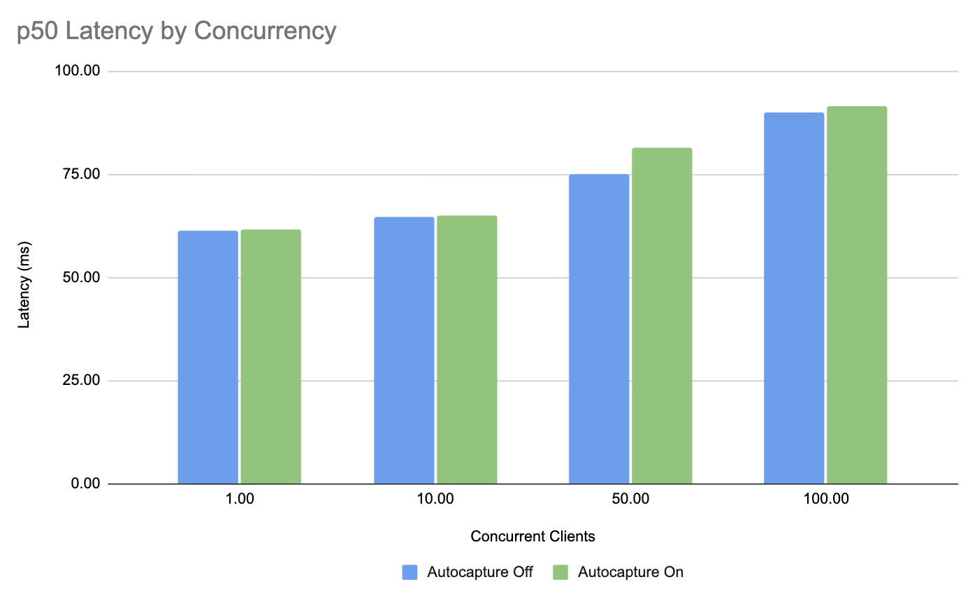
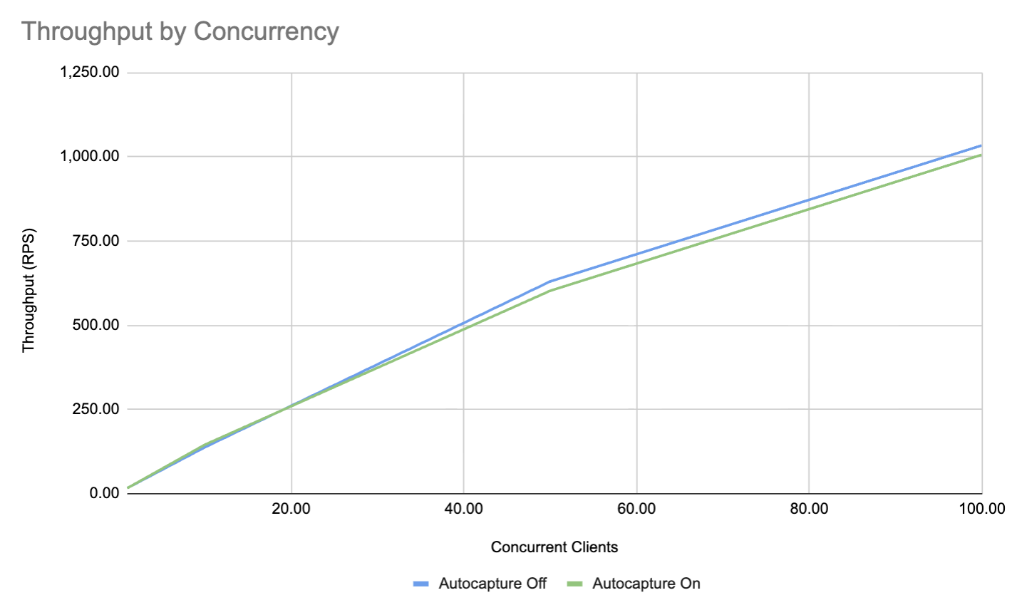
We conducted empirical evaluations to assess the performance impact of automated capture using an XGBoost classification model deployed on a single CPU_X64_L instance, benchmarking execution metrics across varying levels of request concurrency.
- Latency impact: Activating automated capture introduced an end-to-end median latency increase of <10 ms p50 (Figure 1).
- Throughput variance: Overall transaction throughput varied by <1% across the concurrency benchmark spectrum (Figure 2).
A marginal increase in CPU utilization is expected on serving nodes when automated capture is active, reflecting the continuous streaming of payload data into persistent storage. This compute allocation is designed to support near real-time analytical capabilities while preserving latency and throughput bounds.
Payload governance and access control
Automated capture stores transaction records under the model’s native role-based access control (RBAC) definitions, so only authorized principals are permitted to query stored payloads.
To enable asynchronous join operations with ground-truth records, pass an identifier, such as a transaction ID, as a custom attribute. Model owners retain full visibility into raw sensitive attributes transmitted during inference.
Ground-truth label acquisition
Distributional drift metrics quantify variations in input features and model predictions. However, formal performance evaluation (for example, Accuracy, Precision, F1-score, RMSE) necessitates ground-truth labels, which rarely arrive synchronously at inference time. For example, financial fraud labels may materialize hours post-transaction, whereas customer attrition indicators may take several weeks to resolve.
To accommodate delayed labeling, an enterprise-managed ground-truth table can be linked via unique transaction identifiers captured during inference. As ground-truth records land in storage, monitoring tasks continuously ingest the new data to update analytical metrics.
This ground-truth table is integrated into a monitoring object via the GROUND_TRUTH and ID_COLUMNS properties, as detailed in the Evaluation section. This step is optional; if you don’t provide ground-truth labels, the monitor skips performance metrics.
Quantitative evaluation: model-aware observability
Logging predictions is only useful if you can measure whether the model is performing well, by using the right metrics specific to the ML task. Snowflake Model Monitoring dynamically adapts to the ML task defined in Model Registry — binary classification, regression or multiclass classification — and automatically computes the target drift and performance metrics tailored to the model type. Users do not need to specify which metrics to track; the monitoring engine automatically derives the appropriate statistical evaluation suite based on the schema of the registered model version, as shown in the table below, minimizing manual configuration requirements.
| Model type | Drift metrics | Performance metrics (when labels exist) |
|---|---|---|
| Binary classification | Jensen–Shannon, PSI, Wasserstein†, Difference of Means† | Accuracy, Precision, Recall, F1, ROC-AUC‡ |
| Regression | Jensen–Shannon, PSI, Wasserstein, Difference of Means | RMSE, MAE, MAPE, MSE |
| Multiclass classification | Jensen–Shannon, PSI | Accuracy, Macro/Micro Precision & Recall |
| † Wasserstein and Difference of Means need continuous scalars; for binary classification they run on prediction scores, not classes. They do not apply to multiclass. ‡ F1 and ROC-AUC assume a binary positive/negative framework; they do not natively apply to multiclass. |
||
Architectural mechanics of model observability
Snowflake optimizes monitoring compute efficiency by maintaining preaggregated metric tables covering feature distributions, predictive accuracy and subpopulation segments. These structures utilize probabilistic data structures to enable scalable drift computation, preventing the need to rescan raw transaction logs during evaluation cycles.
To establish observability for a deployed model version, construct a source relational view over the raw inference table — flattening nested payload fields and joining ground-truth labels where available — and instantiate a model monitor object.
You can use Snowflake CoCo to generate both the source view and the DDL command for creating the model monitor:
"The fraud detection model FRAUD_DETECTION_MODEL version V1 operates with automated capture active. Predictions include a PRED_CLASS column. A corresponding ground-truth table, FRAUD_GROUND_TRUTH, records late-arriving labels joined on a unique transaction ID stored as a custom attribute. Configure a source view and model monitor with an hourly refresh schedule over a two-day aggregation window."
The resulting command is as follows. First, to create the source view, the monitor expects a flattened schema. The source view performs the flattening step.
# Create the source view: generates a flattened view from the inference table
# (flattens predictions, LEFT JOINs ground truth on your captured ID)

inf_df = session.sql("""
    SELECT
        RECORD_ATTRIBUTES['snow.model_serving.request.extra_columns.TRANSACTION_ID']::VARCHAR AS TRANSACTION_ID,
        RECORD_ATTRIBUTES['snow.model_serving.response.data.PRED_CLASS']::NUMBER              AS PRED_CLASS,
        TIMESTAMP
    FROM TABLE(INFERENCE_TABLE('FRAUD_DETECTION_MODEL', MODEL_VERSION => 'V1'))
    WHERE RECORD_ATTRIBUTES['snow.model_serving.function.name']::VARCHAR = 'predict'
""")

gt_df = session.table("FRAUD_GROUND_TRUTH")

source_view = (
    inf_df.join(gt_df, inf_df["TRANSACTION_ID"] == gt_df["TRANSACTION_ID"], "left")
          .select(
              inf_df["TRANSACTION_ID"],
              inf_df["PRED_CLASS"],
              inf_df["TIMESTAMP"],
              gt_df["LABEL_CLASS"],
          )
)

source_view.create_or_replace_view("FRAUD_MONITOR_SOURCE")
Next, create the model monitor with the FRAUD_MONITOR_SOURCE source view. The REFRESH_INTERVAL controls how often new predictions are ingested. AGGREGATION_WINDOW controls how far back the drift and performance metrics look. Setting a two-day window here means each hourly refresh recalculates metrics over a rolling 48-hour slice of predictions. For our fraud detection example, this means that the refresh is recent enough to catch degradation quickly, yet wide enough to smooth out low-traffic periods.
# Create model monitor with the source view

from snowflake.ml.monitoring.entities.model_monitor_config import ModelMonitorConfig, ModelMonitorSourceConfig

source_config = ModelMonitorSourceConfig(
    source="FRAUD_MONITOR_SOURCE",
    timestamp_column="TIMESTAMP",
    id_columns=["TRANSACTION_ID"],
    prediction_class_columns=["PRED_CLASS"],
    actual_class_columns=["LABEL_CLASS"],
    baseline="FRAUD_DETECTION_BASELINE",
)
monitor_config = ModelMonitorConfig(
    model_version=reg.get_model("FRAUD_DETECTION_MODEL").version("V1"),
    model_function_name="predict",
    background_compute_warehouse_name="MY_WAREHOUSE",
    refresh_interval="1 hour",
    aggregation_window="2 days",
)
monitor = reg.add_monitor("MY_VERSION_MONITOR", source_config, monitor_config)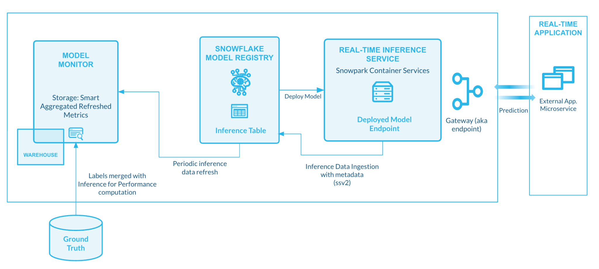
Model promotion and controlled deployment strategies: traffic splitting, shadowing
Now that you have logged the predictions and monitored them, you need a way to test and validate new candidate model versions on real traffic before deploying them.
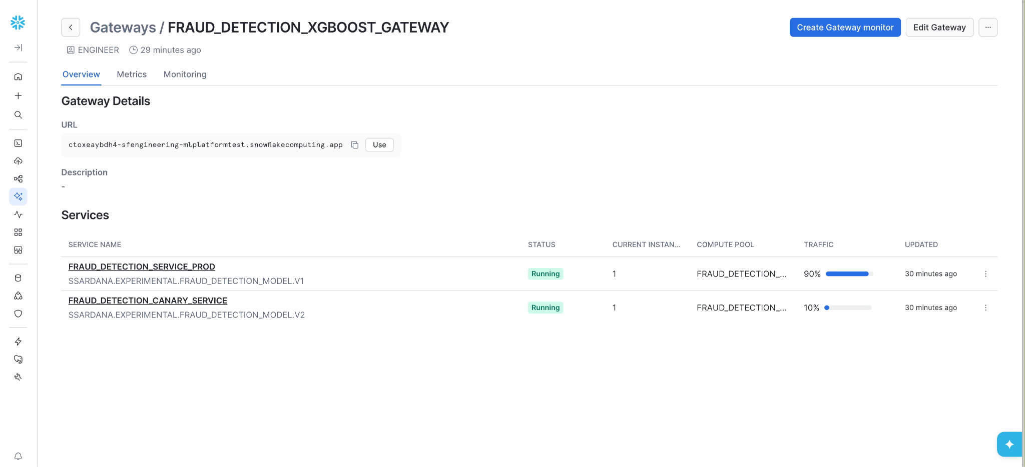
A Gateway solves this problem by serving as an abstraction layer fronting one or more backing model services. Client applications interface with a single, persistent endpoint URL while the gateway enforces configured traffic allocation policies. Consequently, model updates no longer require coordinated client-side changes.
session.sql("""
    CREATE GATEWAY FRAUD_DETECTION_XGBOOST_GATEWAY FROM SPECIFICATION $$
    spec:
      type: traffic_split
      split_type: custom
      targets:
      - type: endpoint
        value: mydb.myschema.FRAUD_DETECTION_SERVICE_PROD!inference
        weight: 90
      - type: endpoint
        value: mydb.myschema.FRAUD_DETECTION_CANARY_SERVICE!inference
        weight: 10
    $$
""").collect()
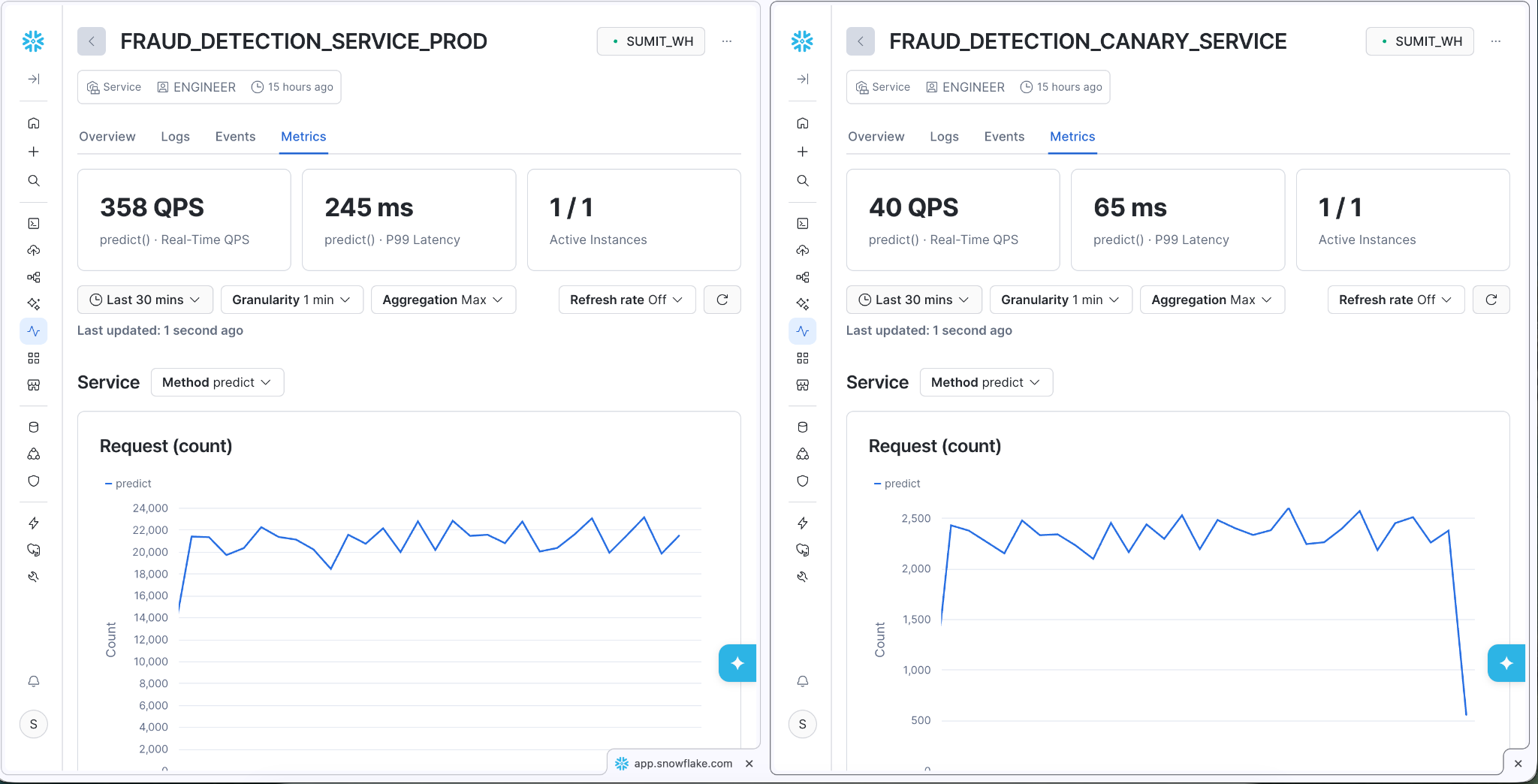
Traffic splitting: Routes a defined proportion of live requests to a candidate model (for example, 10%) while the baseline version processes the remaining volume. Both deployments handle live requests and write transaction records to their respective inference tables. This allows users to compare on live traffic distribution and scale up traffic allocation iteratively (for example, 10/90 → 30/70 → 100/0) as empirical confidence increases.
Shadow deployments: Shadow deployments (in public preview) are used for evaluating candidate performance against production traffic distributions without impacting client-facing applications. It asynchronously duplicates incoming production traffic and replays the requests against a candidate service. Candidate predictions are logged exclusively for offline comparison rather than returned to the client, so production users see only the primary service’s response.
Evaluating A/B testing results
A Version Monitor tracks a single deployed model version. Conversely, a Gateway Monitor dynamically inspects all active service endpoints configured behind a gateway, applying uniform monitoring principles to facilitate live comparative A/B testing.
A Gateway Monitor can be created using the Snowflake CoCo prompt:
"Construct a Gateway Monitor named FRAUD_AB_MONITOR for FRAUD_DETECTION_MODEL operating behind FRAUD_DETECTION_XGBOOST_GATEWAY. Track drift metrics across all attached services with an hourly refresh schedule over a one-hour aggregation window using warehouse MY_WAREHOUSE. Integrate FRAUD_GROUND_TRUTH joined on TRANSACTION_ID to evaluate classification accuracy over a 24-hour window."
Leading to the following DDL:
session.sql("""
    CREATE MODEL MONITOR MY_GATEWAY_MONITOR
    WITH
      MODEL      = 'FRAUD_DETECTION_MODEL'
      GATEWAY    = 'FRAUD_DETECTION_XGBOOST_GATEWAY'
      FUNCTION   = 'predict'
      WAREHOUSE  = MY_WAREHOUSE
      REFRESH_INTERVAL   = '1 hour'
      AGGREGATION_WINDOW = '24 hours'
      GROUND_TRUTH = FRAUD_GROUND_TRUTH
      ID_COLUMNS = ('TRANSACTION_ID')
      ACTUAL_CLASS_COLUMNS    = (LABEL_CLASS)
      PREDICTION_CLASS_COLUMNS = (PRED_CLASS)
""").collect()
The instantiated monitor calculates drift indices and system metrics prior to the arrival of ground-truth labels. As records accumulate within the ground-truth relation, performance metrics automatically re-evaluate during subsequent refresh cycles. In the absence of ground-truth data, feature and prediction drift calculations continue to function independently.
Gateway Monitors support aggregation windows as short as one hour, enabling rapid evaluation during live experiments. In low-volume candidate traffic splits (for example, 10%), statistical confidence intervals around candidate performance metrics remain relatively wide. Promotion decisions require demonstrating not only higher point-estimate performance, but also that these intervals have sufficiently narrowed to confirm significance.
During active A/B testing, each gateway target independently aggregates joined outcome labels, delivering statistically rigorous comparative assessments to guide promotion decisions. Predictive performance gains must be evaluated alongside system-level efficiency. A candidate model showing superior predictive accuracy may nevertheless be unsuitable for promotion if it introduces excessive latency, elevated memory overhead or instability under load. Gateway Monitoring consolidates transaction rates, error frequencies, latency percentiles, CPU usage and memory consumption into unified dashboards alongside data drift and accuracy metrics. Promotion criteria should dictate that model quality gains be verified concurrently with infrastructure stability.