How Snowflake Optima Planning Cut a Query from 219s to 3s


In a production workload, Optima Planning sped up a query from 219 seconds to 3 seconds — 73× faster — one of the larger gains we observed, by measuring a filter's actual selectivity from data samples before execution.
Snowflake Optima automatically improves workload performance without requiring customers to tune, configure or maintain optimization structures. Optima Planning is the part of Optima that improves query plan quality by grounding optimizer decisions in real workload evidence. Optima Planning learns from query executions: for example, recognizing joins that exploded on a previous run and correcting their cardinality on the next one.
Execution history is a powerful signal, but it is reliable only when a query's behavior stays stable from one run to the next. When a filter's selectivity changes abruptly, what happened last time no longer predicts what the optimizer will face this time. This is especially true for predicates whose selectivity is hard to pin down: complex LIKE filters, predicates that wrap a column in a function (built-in or user-defined, a UDF) and filters correlated across multiple columns.
For those cases, Optima Planning now uses dynamic sampling: a small, bounded compile-time read of the relevant data to validate uncertain cardinality estimates each time the query is compiled. The result is plan choices that are designed to adapt to what the data actually looks like right now, not only to what past executions showed, with no customer configuration required.
TL;DR: Snowflake Optima Planning uses dynamic sampling, which is designed to deliver faster query latency for workloads with uncertain, shifting selectivity: before the optimizer commits to a plan, it checks an uncertain cardinality estimate against a small, bounded read of real historical data—most useful for filters whose selectivity changes from one execution to the next.
Optima Planning: Better evidence, better plans
Snowflake Optima extends Snowflake's core principles of performance and simplicity by continuously analyzing workload patterns and applying optimization strategies automatically. The goal is simple: make queries run faster and more cost-efficiently, without requiring customers to configure or maintain tuning structures.
Optima Planning focuses specifically on query plan quality. It continuously observes how queries run, captures information from execution, and uses that information to make better planning decisions for future executions. This is especially powerful for recurring workloads such as dashboards, scheduled reports and ELT pipelines.
Runtime feedback answers an important question:
> What happened last time this workload ran?
Dynamic sampling answers a complementary question:
> What does the relevant data actually look like right now?
Together, they help keep the optimizer's estimates grounded in reality, learning about exploding joins from past executions while adapting to filters whose selectivity changes from run to run.
What is Dynamic Sampling?
Dynamic sampling is a targeted, compile-time technique in Optima Planning that reads a small, bounded sample of the relevant data to check an uncertain filter estimate before the optimizer picks a plan. It targets predicates whose selectivity is hard to characterize from summary statistics alone — complex LIKE filters, function-wrapped predicates and multicolumn correlations — and activates only for queries large enough to be worth checking.
How Dynamic Sampling works
Today, Optima Planning uses dynamic sampling to measure filter selectivity — how many rows a filter actually keeps. At a high level:
- For a query expensive enough that a planning mistake would cost more than the sample, Optima Planning finds a filter whose selectivity is uncertain.
- It applies that filter to a small, bounded sample of real data and measures how many rows actually survive.
- The corrected estimate feeds back into planning, so the optimizer chooses its plan with evidence instead of a guess.
The important part is that this happens before execution.
Dynamic sampling does not replace runtime feedback. It is intended to complement it, filling in for cases where past executions can't tell you what this run's data looks like, so the plan adapts even when this run's selectivity differs from what earlier runs showed.
Why estimates matter
Snowflake's optimizer is cost-based. For every query, it considers candidate plans, estimates how many rows each operator will produce, and chooses the plan expected to be cheapest.
When those estimates are accurate, the chosen plan is usually optimal or the best fit for the workload.
However, when those estimates are suboptimal, the consequences can be enormous. A filter that looks broad but is actually highly selective can change the right join order, the right build side of a hash join and the amount of intermediate data the engine needs to process. One bad estimate early in a plan can cascade into billions of unnecessary intermediate rows downstream.
When statistics are not enough
Most summary statistics are designed to characterize columns. But SQL predicates often operate on meaning, not just columns.
These are the cases where dynamic sampling helps. In each one the predicate is typically parameterized ( the literal value changes from one run to the next) so even a prior execution of the same query shape can have a very different selectivity, and execution history alone cannot predict this run:
Complex LIKE filters
description LIKE :pattern // '%return%' one run, '%urgent shipment%' the nextA wildcard pattern's match rate depends on the actual string contents of the column, and the pattern itself changes from run to run. Per-column statistics such as min/max and distinct counts cannot describe how many rows a given pattern will match, and last run's pattern says nothing about this one's.
Predicates that wrap a column in a function (built-in or UDF)
DATE_TRUNC('month', order_ts) = :month   // a different month each run
MY_UDF(col_a, col_b) = :flag
Per-column statistics describe the base column, but not the result of an arbitrary function applied to it — whether built-in or user-defined. An incremental pipeline may select a quiet month (2% of the rows) on one run and a peak month (30%) on the next, so the slice the filter returns shifts every execution.
Filters correlated across multiple columns
WHERE make  = :make    -- a different make/model
  AND model = :model   --   pair each run
Per-column statistics treat the two filters as independent and multiply their selectivities, under-estimating the rows the query returns whenever the columns are correlated (every Corolla is a Toyota, so model already implies make). The specific pair changes from run to run, and a common pair returns far more rows than a rare one, so the size of the error shifts with each execution. Those cross-column relationships are hard to capture with per-column statistics in the first place.
In all of these, the optimizer would plan better with direct evidence about the data, which is what dynamic sampling provides.
A synthetic example: Row skew and functions
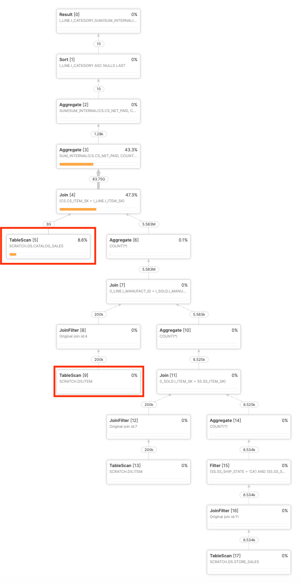
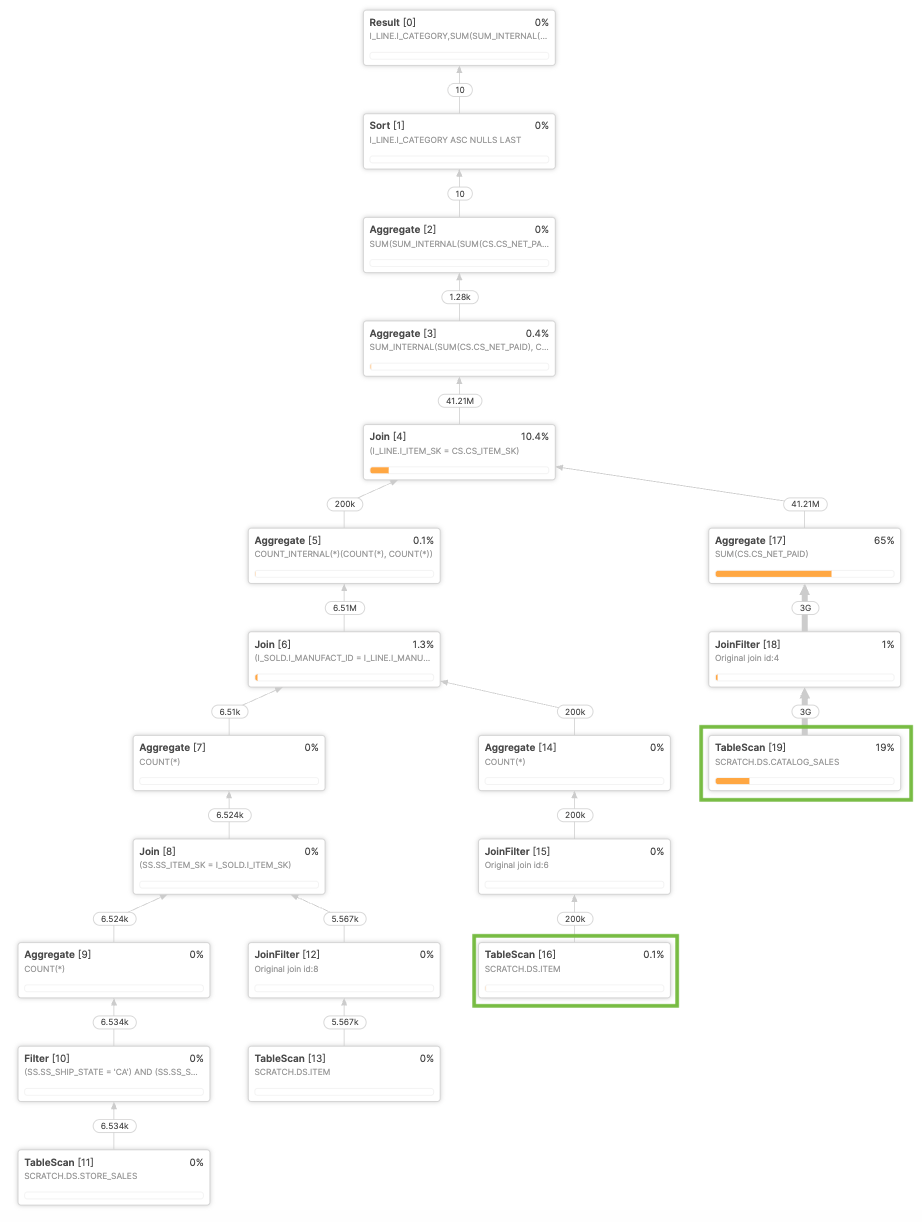
This query's plan hinges on getting three predicates right, and two of them are exactly the kind summary statistics miss. Consider a cross-channel merchandising query over a TPC-DS-style schema: for a narrow segment of in-store purchases (those in a recent date window, shipped to San Francisco, California, and limited to a 1% sample of customers), it looks up the manufacturer of each item bought and totals the catalog-channel revenue of that manufacturer's entire product line, broken down by product category. The query plan depends on the selectivity of the filter applied to the store_sales fact, which combines three predicates with very different estimation characteristics: a date-range predicate, which Snowflake's already estimated well; a correlated pair of predicates (ship_state = 'CA' and ship_city = 'San Francisco'), where the optimizer's independence assumption misjudges the true selectivity because the two columns are related; and a modulo expression used to sample customers, whose selectivity can't be derived from any single-column statistic. The optimizer misestimates how many rows survive the filter because it can't see either problem, the same correlation and function limitations explained below. Because that bad estimate feeds the join planning, the optimizer places the large catalog_sales table on the build side of the topmost join and the highly selective store_sales on the probe side of the bottommost join, an expensive plan. Dynamic sampling runs a small sample of that filter at compile time, measures its true selectivity, and feeds the corrected cardinality back into the optimizer. With an accurate estimate, the optimizer flips the join order: it places the tiny store segment first on the build side and the large catalog sales table on the probe side, returning the same result with far less work.
Why doesn't a conventional histogram rescue this plan on its own? A histogram-based approach can estimate the distribution of values within a single column, and for the date-range predicate that's enough. But histograms are inherently per-column, and the other two predicates defeat them in two different ways. The ship_state/ship_city pair is a correlation problem: a histogram on state and a histogram on city are each individually correct, yet neither reveals that San Francisco sits entirely within California. The modulo predicate is a function problem: a histogram on customer_sk describes the customer ids themselves, but tells you nothing about the selectivity of customer_sk % 100 = 0. Dynamic sampling can sidestep both issues: it evaluates the actual predicate against a small sample of real rows at compile time, so it learns the true combined selectivity that no per-column histogram could express.
select i_line.i_category, sum(cs.cs_net_paid) as manufacturer_line_catalog_revenue
from store_sales ss
join item i_sold  on ss.ss_item_sk = i_sold.i_item_sk
join item i_line  on i_line.i_manufact_id = i_sold.i_manufact_id
join catalog_sales cs on cs.cs_item_sk = i_line.i_item_sk
where ss.ss_sold_date_sk between 3370 and 3399
  and ss.ss_ship_state = 'CA' and ss.ss_ship_city = 'San Francisco'
  and mod(ss.ss_customer_sk, 100) = 0
group by i_line.i_category
order by i_line.i_category;
*Sample query on TPC-DS Data. Warehouse size is X-LARGE. Table sizes are 200K, 1B, and 3B rows.
We can see the query plan change with dynamic sampling. The total duration of the query (including the overhead of dynamic sampling) decreases from 37.0s to 2.3s, a 16x improvement. Dynamic sampling is not tied to specific filter values. You can change the filter values, and dynamic sampling will still apply. The two plans below show the query before and after dynamic sampling, respectively.
A production example
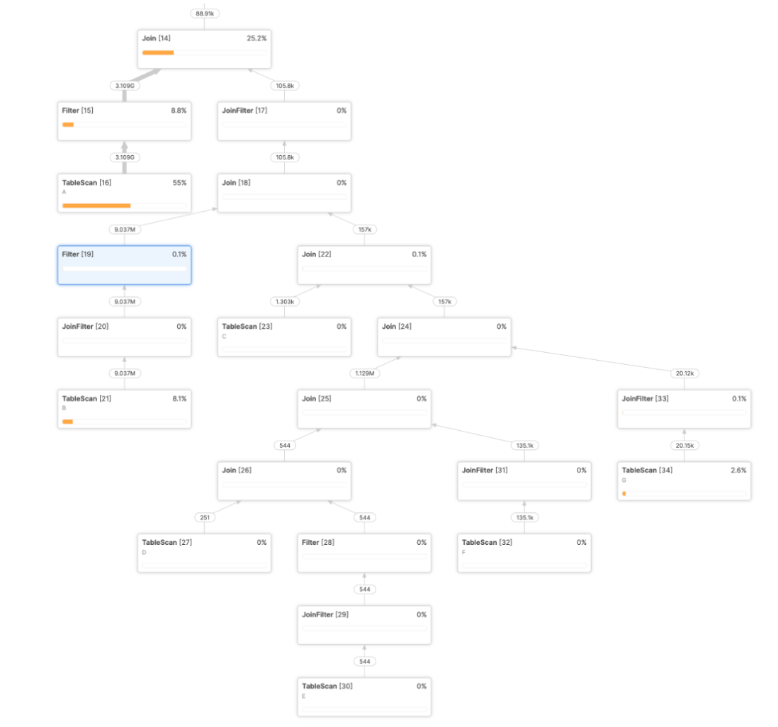
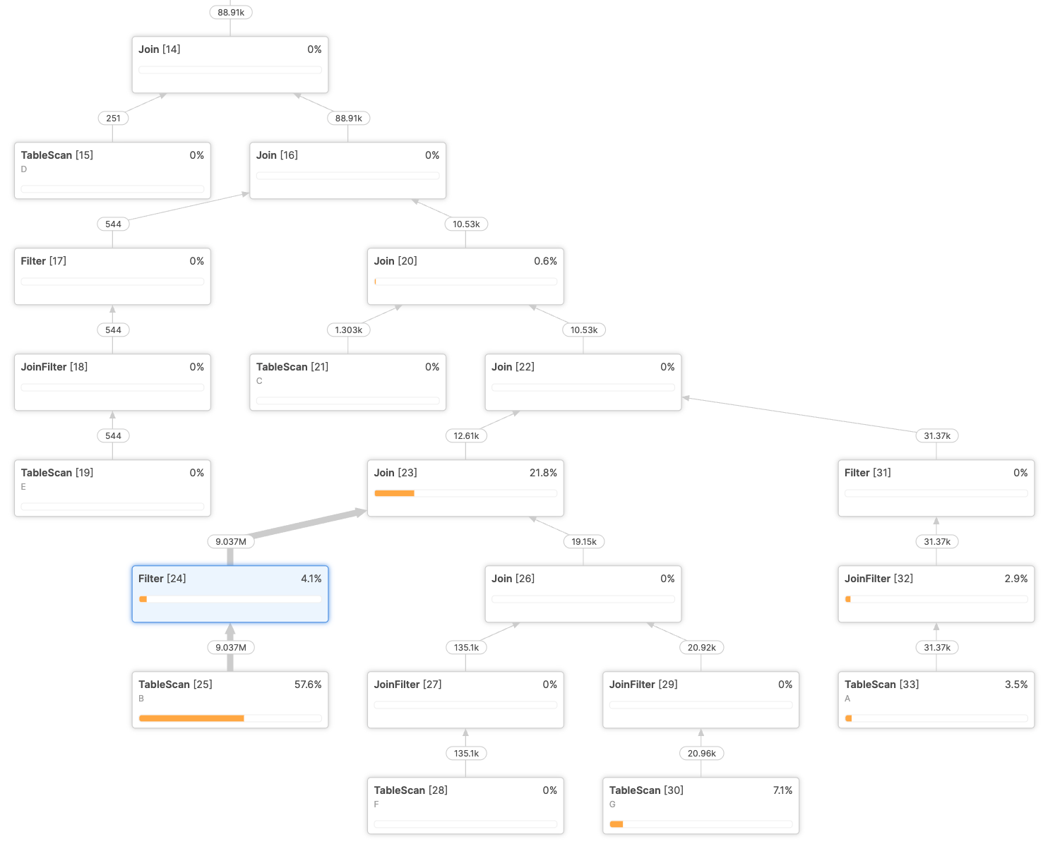
We've seen this improvement in real customer workloads too. In the example below, a customer's query improved from 3m39s to 3s, a 73x improvement. The optimizer over-estimated the highlighted filter above table labeled B, which pushed the join order into an expensive shape; dynamic sampling corrected the estimate, and the optimizer re-ordered the joins, scanning fewer rows on several tables as a result. Snowflake has redacted the query plan to hide customer details.
Both examples above are among the larger improvements we've seen; see "Where Dynamic Sampling does not help" below for where the gain is smaller, or the optimizer already had it right.
When Dynamic Sampling helps
Dynamic sampling is most valuable when summary statistics are insufficient and selectivity shifts from run to run. By sampling at compile time, Optima Planning adapts the plan to current data instead of relying solely on past executions. It helps most when:
- the query is expensive enough that a bad estimate would trigger large scans or joins
- the filter is a complex LIKE, a function-wrapped predicate (built-in or UDF) or a multicolumn correlation
- selectivity shifts between runs, as with parameterized or date-range and incremental-load filters
- the SQL is freshly generated by BI tools or LLMs (for example, Cortex Analyst, Tableau Pulse)
- the workload is migrated from Teradata, Oracle, or DB2, with unfamiliar encoding conventions and predicate shapes
These are the cases where better compile-time evidence can materially improve the plan.
Where Dynamic Sampling does not help
Dynamic sampling is not a universal accelerator. It does not meaningfully improve workloads that already plan well from existing statistics. For example:
- small, inexpensive queries where sampling would not pay for itself
- simple equality filters on well-characterized columns
- recurring dashboards already improved by runtime feedback
- queries where the optimizer's estimates are already accurate
- workloads where the bottleneck is not cardinality estimation
In those cases, Optima Planning either uses other mechanisms or leaves the plan unchanged.
That is by design. Dynamic sampling is targeted at cases where better compile-time evidence can materially improve the plan.
How customers can observe Optima
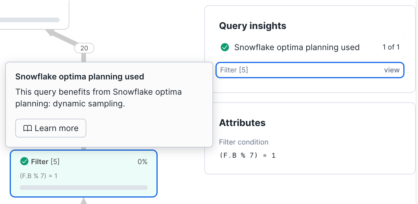
Customers can monitor Snowflake Optima use in Query Profile under Query History, including the Query insights pane and Statistics pane. Snowflake also exposes Optima-related information through the QUERY_INSIGHTS view.
For Optima Planning specifically, this means customers can see when Snowflake has applied optimization insights to improve plan quality. For instance, if dynamic sampling was used, the insight will explicitly state: "This query benefits from Snowflake optima planning: dynamic sampling."
Key takeaways
Optima Planning is about better evidence for better plans.
Snowflake learns about exploding joins from previous executions through runtime feedback, and measures how a filter behaves on the current data through dynamic sampling.
Together, these mechanisms cover more of the workload lifecycle:
- Recurring workloads: dashboards, scheduled reports and ELT pipelines improve as Optima Planning learns about exploding joins from past executions.
- Dynamically changing filters: date-range and incremental-load predicates, and other filters whose selectivity changes from run to run, are measured directly by compile-time sampling.
- Complex predicate workloads: LIKE expressions, function-wrapped predicates (built-in or UDF) and multicolumn correlations can be planned more accurately when summary statistics are not enough.
In production, this translated into a customer query improving from 219 seconds to 3 seconds, 73x faster, which is one of the larger gains we observed, by measuring a filter's actual selectivity from data samples before execution.
No manual tuning. No manual configuration. Just better plans.
*This post may contain forward-looking statements about future product capabilities. Actual results may differ. See our latest 10-Q."
Related:
- Snowflake Optima documentation
- Snowflake Optima Planning
- Snowflake Cortex AI
- Snowflake Performance Improvements release notes: month-by-month list of shipped optimizations
- Snowflake Performance Index: methodology and weekly improvements
- Snowflake Engineering Blog: for the broader cadence of performance posts