Jul 16, 2026/10 min readMachine Learning
How Snowflake Solves Batch Inference Bottlenecks to Deliver 6.5x Higher Throughput


Batch inference, while conceptually straightforward—involving the execution of a model over a data set to generate results—presents significant engineering challenges when implemented at scale. Typically, the primary bottleneck resides not within the model itself, but in the surrounding infrastructure, encompassing data movement, serialization, scheduling and resource management. These elements determine both the efficiency of the job's execution and its associated computational costs. Ultimately, maximizing throughput — defined as the volume of rows processed per second — is essential for optimizing performance and cost-efficiency.
Batch Inference Jobs in Snowflake ML solves exactly that with a simple managed API:
registry = Registry(session=session, database_name=DATABASE, schema_name=REGISTRY_SCHEMA)
mv = registry.get_model('my_model').version('my_version')  # returns ModelVersion

# how to run a batch job
job = mv.run_batch(
    compute_pool = "my_compute_pool",
    X = session.table("my_table"),
    output_spec = OutputSpec(stage_location="@my_db.my_schema.my_stage/path/"),
)

job.wait() # Optional: Blocking until the job finishes
This solution is decoupled from traditional SQL constraints, engineered to optimize the large-scale processing of unstructured data and file-based data sets. The platform facilitates fully automated distributed execution—encompassing partitioning, scheduling, resource management and automated teardown. For inline predictions within SQL pipelines, users should use native batch inference functions, while real-time application backends should leverage service endpoints.
We conducted a comparative analysis of Batch Inference Jobs against Databricks Spark UDF and Amazon SageMaker Batch Transform using equivalent CPU configurations (RAM differed but was not a bottleneck; see Methodology). Our results indicate that on the tested workloads, Snowflake's run_batch() API delivered up to 6.5x higher throughput and up to 5.8x lower compute cost per million rows compared to SageMaker Batch Transform and Databricks Spark UDF.
What we tested
The evaluation encompassed two distinct categories of models, selected to represent divergent workload profiles:
- Structured Models (XGBoost): Characterized by structured input and output formats, these models are CPU-intensive and facilitate rapid per-row inference. The primary engineering objective involves optimizing raw throughput and ensuring the system provides data at a rate sufficient to sustain the model's processing capacity.
- Embedding Models (Sentence Transformer): These models transform unstructured text into structured embedding vectors. They are GPU-intensive and exhibit comparatively slower per-row inference. The central challenge lies in achieving and maintaining effective GPU utilization rather than mere saturation.
We compared three platforms, each with a different architecture for batch inference:
- Snowflake Batch Inference Jobs — Managed batch inference on Snowpark Container Services (SPCS). Specify compute pool and model; scheduling, partitioning and teardown are handled automatically.
- Databricks Spark UDF — Apply a Python UDF containing inference logic to a Spark DataFrame. Requires managing a Spark cluster and submitting a job to it.
- Amazon SageMaker Batch Transform — Send batched S3 payloads to a dedicated offline inference container via a SageMaker transform job.
Benchmarks
Methodology and evaluation framework
- All fiscal evaluations utilize public on-demand pricing models:
- Snowflake — SPCS compute credits per hour
- Databricks — VM instance cost + Databricks Unit (DBU) markup per hour
- SageMaker — Hourly per-instance pricing
- The reported findings represent median values derived from three independent experimental iterations.
- XGBoost needs 10 billion rows because its near-zero cost per row requires massive volume to expose platform overhead. Conversely, the compute-bound Sentence Transformer stabilizes throughput and cost metrics at 10 million rows. Scaling embedding data sets further only increases execution time—already approximately one hour on the slowest platform—without altering per-row metrics.
- CPU configurations were systematically standardized across all evaluated platforms. RAM was not standardized as it was not a bottleneck on the specific workloads and platforms evaluated. Additionally, execution runtimes were quantified server-side to eliminate confounding variables associated with client-side latency.
- The financial evaluation is strictly confined to computational resource consumption, explicitly excluding expenditures associated with data storage, orchestration, or egress operations.
Comparative performance analysis
XGBoost
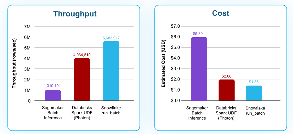
Cost calculation included in the appendix below - section A
Sentence Transformer (Embedding model)

Cost calculation included in the appendix below - section B
These benchmarks evaluate distinct system performance drivers. The XGBoost test, conducted at extreme scale, highlights the importance of efficient data handling: Arrow-native processing, directed acyclic graph (DAG) fusion, and optimized batching minimize overhead. Conversely, the Sentence Transformer test demonstrates that GPU utilization determines performance when compute is the primary constraint; success requires decoupling I/O from inference and sizing batches to VRAM capacity. On matched CPU configurations, Snowflake Batch Inference Jobs achieved up to 6.5x higher throughput and up to 5.8x lower compute cost per million rows in our benchmarks, compared to SageMaker Batch Transform and Databricks Spark UDF. The following analysis details these performance optimizations.
Under the hood: What drives the performance
Continuous profiling of our batch inference execution enabled significant pipeline optimizations. We increased XGBoost throughput from 1.4M rows/s on 1B rows to 5.68M rows/s on 10B rows, primarily through the amortization of fixed startup costs. These improvements leverage the Ray Data execution architecture, which optimizes throughput by fusing adjacent logical operators into single physical units, thereby minimizing intermediate data materialization.
DAG compression and fusion
Ray Data uses operator fusion to optimize execution, though achieving maximum efficiency requires an intentionally architected DAG. To ensure an optimal streaming pipeline and prevent the introduction of materialization barriers, we employ two primary optimization techniques:
- Data Processing Consolidation: By performing signature normalization and column mapping directly within the actor's batch function, we eliminate standalone operators. This ensures transformations remain within the execution context, preventing fusion boundary breaks that stall the pipeline.
- Resource Requirement Alignment: Adjacent operators must share identical resource requests (e.g.,
num_cpus). Divergent resource declarations preclude Ray from merging logical units into a single physical operator, thereby disrupting the fusion chain.
Implementing these methods maintains a fully fused pipeline, reducing the architecture from five stages with four object-store boundaries to three streaming stages with zero full-dataset materialization barriers.
Resource tuning
Ray's resource declarations function as scheduling constraints rather than strict capacity limits. To optimize performance, we implement a two-part resource management strategy:
- Maximize I/O Concurrency: For I/O-bound operations (e.g., stage read/write), we declare minimal CPU requirements (e.g.,
num_cpus=0.01). This prevents the scheduler from throttling I/O, allowing full saturation of network bandwidth and continuous data availability. - Optimize Inference Allocation: Inference actors require precise compute allocations to ensure efficient batch processing. Under-declaring throttles parallelism, while over-declaring risks resource contention and out-of-memory (OOM) errors. We align resource definitions with the model's actual footprint to maintain consistent throughput and prevent contention.
Arrow-native processing
Machine learning frameworks, such as XGBoost and Scikit-Learn, typically require inputs as Pandas DataFrames. However, a technical mismatch exists between Pandas' single-machine, in-memory orientation and Ray Data's distributed, high-throughput architecture, which utilizes Apache Arrow's columnar memory format. Automated Arrow-to-Pandas conversion—specifically via standard map_batches(batch_format="pandas") configurations—introduces significant overhead. Executing structural operations, such as column renaming, type casting, and subset selection, within the Pandas environment triggers redundant memory allocations and data copies.
To mitigate this, we implemented an "Arrow-native" approach. We perform all structural transformations within the Arrow memory space, leveraging zero-copy operations to avoid unnecessary overhead. The conversion to Pandas is deferred until the final execution step, restricted strictly to the columns required by the model.

Arrow tables are metadata wrappers around independent column buffers. "Concatenating" two tables horizontally just creates a new metadata object whose column list points to the original buffers — no bytes move. Pandas DataFrames, by contrast, typically allocate new memory and copy column buffers into the result. For a pipeline doing millions of these merge operations, the difference compounds fast.
Optimal batch sizes
Inference actors process data in batches, necessitating normalization and conversion for each subset. Amortizing the fixed overhead per batch is essential for performance; processing thousands of rows in a single batch is significantly more efficient than performing the same operations sequentially. The relationship between overhead and batch size is defined as:
Total Overhead ≈ (Total Rows / Batch Size) × Fixed Batch Overhead
Increasing the batch size reduces the total number of batches, thereby minimizing overhead. This principle applies to both data preprocessing and model inference, where larger batches improve throughput by distributing fixed costs across more rows. The primary constraint for increasing batch size is peak memory utilization (RAM and VRAM). As demonstrated in the XGBoost case study, where per-row inference latency is minimal, establishing a sufficient batch size is critical to amortize platform overhead effectively.

1B XGBoost rows, eight replicas, five workers. Same workload — only batch size changes. Read/write time is excluded.
At a batch size of 1,024, Inference Actor execution time is predominantly consumed by pre- and post-processing rather than model inference. Scaling to a batch size of 16,384 prioritizes inference compute, maximizing throughput. However, throughput gains eventually plateau as memory consumption scales linearly.
Optimal batch sizing is inherently workload-dependent. Structured models, characterized by minimal per-row footprints, accommodate large batch sizes. Conversely, GPU-accelerated models (e.g., embedding, vision) are constrained by activation memory and token limits, necessitating moderate batching.
| Model Type | Batch Size | Order of Magnitude |
|---|---|---|
| Structured | Larger | 10k-50k rows |
| Unstructured | Smaller | 1k-10k rows |
Table 1: Optimal batch sizes by Model Type
Combined effect
The platform achieves superior throughput through four integrated optimizations that are designed to eliminate processing bottlenecks:
- DAG Fusion: Merges logical operators into a single physical execution unit, eliminating intermediate materialization barriers and preventing pipeline stalls.
- Resource Tuning: Decouples I/O from inference requirements, enabling concurrent execution without artificial scheduler throttling.
- Arrow-Native Processing: Leverages Apache Arrow to perform structural transformations via zero-copy operations, significantly reducing invocation overhead compared to Pandas-based workflows.
- Optimal Batch Sizing: Amortizes fixed execution costs by increasing batch sizes to maximize compute utilization, reducing the total number of required actor invocations.
The benchmarks reported above include all four optimizations, and we continue to profile and push throughput further.
Get started
To implement batch inference workloads in Snowflake ML, consult the Batch Inference Jobs documentation. Configure the run_batch operation by specifying the target model and compute pool; the platform manages the remaining infrastructure. To begin, execute the benchmarks using our reference notebooks: XGBoost and Sentence Transformer.
Appendix
Pricing reference
All costs use public on-demand pricing. Credit-to-dollar conversion: $2.36/credit.
| Benchmark | Platform | Instance Type | Nodes | Hourly Rate |
|---|---|---|---|---|
| XGBoost | Snowflake | CPU_X64_M (4 of 6 vCPU, 28 GiB) | 8 | 0.22 credits/node |
| XGBoost | Databricks | Standard_D4ds_v5 (4 vCPU, 16 GiB) | 8 | $0.376/node |
| XGBoost | SageMaker | ml.m5.xlarge (4 vCPU, 16 GiB) | 8 | $0.23/node |
| Sentence Transformer | Snowflake | GPU_NV_XS (T4, 16 GiB GPU) | 2 | 0.25 credits/node |
| Sentence Transformer | Databricks | Standard_NC4as_T4_v3 (T4, 16 GiB GPU) | 2 | $0.676/node |
| Sentence Transformer | SageMaker | ml.g4dn.xlarge (T4, 16 GiB GPU) | 2 | $0.7364/node |
Table 2: Hardware and Rates
Cost derivations
- XGBoost comparison
- Snowflake:
8 nodes × 0.22 credits/hr × 4/6 × 1,759.37s / 3,600 = 0.573 credits; at$2.36/credit→$1.35total. We limited each node to 4 of its 6 available vCPUs to match the 4-vCPU instances used by SageMaker and Databricks. Cost is prorated accordingly (4/6). - SageMaker:
8 × $0.23/hr × 11,520.95s / 3,600→$5.89total. - Databricks:
8 × $0.376/hr × 2,460.39s / 3,600→$2.06total.
- Snowflake:
- Sentence Transformer comparison
- Snowflake:
2 nodes × 0.25 credits/hr × 792.58s / 3,600 = 0.110 credits; at$2.36/credit→$0.26total. - SageMaker:
2 × $0.7364/hr × 3,670.82s / 3,600→$1.50total. - Databricks:
2 × $0.676/hr × 1,319.26s / 3,600→$0.50total.
- Snowflake: