Accelerating Semantic Views with Materializations

Semantic views give you a single, governed definition of your metrics and dimensions offering one source of truth shared across BI tools, Cortex Analyst and ad hoc Semantic SQL. Just like regular views, Snowflake still computes queries against the base tables, which can result in complex plans and long-running queries on large data sets.

Semantic view materializations fix this using an approach that is similar to materialized views: We precompute semantic view (SV) aggregations and queries that benefit from the materialization are rewritten automatically to use it. This way, SV workloads can run orders of magnitude faster. In contrast to regular materialized views, materializations are specified directly using the dimensions and metrics of the SV.

Snowflake keeps the materialization up to date in the background — bounded by a staleness target you set — and a single materialization can serve many different queries by re-aggregating a fine-grained rollup up to whatever grain each query asks for.

How it works

Prerequisites. Before you can materialize anything, set a freshness bound on the semantic view:

A max_staleness of 1 hour means that we will never return results that are more than one hour stale — materializations that lag behind by more than one hour are not used automatically. This allows us to trade refresh costs and freshness.

Creating a materialization. You declare the dimensions and metrics to precompute and the warehouse that builds and refreshes it:

Staying fresh: Snowflake refreshes the materialization in the background to keep it within MAX_STALENESS, using the warehouse you specified. REFRESH_MODE can be AUTO, FULL or INCREMENTAL; with AUTO, Snowflake picks the mode. You can always force a refresh manually:

How the planner uses it: When you query the semantic view, the planner selects the lowest-cost materialization that covers the requested dimensions and metrics. Two behaviors make one materialization cover a wide range of queries:

• Re-aggregation of additive metrics: A materialization on (customer_name, order_year) with SUM(total_revenue) can answer a query that asks only for customer_name — Snowflake just sums across years. SUM, COUNT, MIN and MAX all re-aggregate this way.
• WHERE-clause dimensions count as covered. A filter like WHERE order_year = 2024 is satisfied directly from the stored rollup, as long as order_year is a materialized dimension (expressions on those dimensions work too).

You can also materialize a filtered subset — for example, just the last two years of orders — by adding a WHERE clause to the materialization. Queries with an equal-or-more-restrictive filter still get accelerated.

Limitations

The single most important constraint is additive vs. non-additive metrics, because it determines whether one rollup can serve many queries:

• Additive metrics — SUM, COUNT, MIN, MAX — can be re-aggregated. A fine-grained rollup serves coarser queries by rolling up across the extra dimensions. This is what makes materializations broadly reusable.
• Non-additive metrics cannot be re-aggregated, so a materialization only helps a query at exactly the stored grain. This includes COUNT(DISTINCT), APPROX_COUNT_DISTINCT, MEDIAN, PERCENTILE_CONT/PERCENTILE_DISC, AVG, any DISTINCT aggregation and derived metrics that reference non-additive metrics. An expression on top of an aggregation (for example, 2*SUM(x)+COUNT(y)) is also not additive.

A few other things to know:

• Only Semantic SQL benefits: Queries through the SEMANTIC_VIEW construct or standard SQL against the semantic view are accelerated. Cortex Analyst, Cortex Agents and CoWork paths that emit physical SQL directly against the base tables do not benefit.
• Base-table scans: A query falls back to a base-table scan when no materialization covers the requested dimensions/metrics; the data exceeds the MAX_STALENESS window; a masking or row-access policy exists on a referenced column; a non-additive metric would need re-aggregation; the materialization is suspended; or the query's WHERE is less restrictive than the materialization's filter (or filters a non-materialized column).
• Auto-suspend on staleness: If MAX_STALENESS is too low for background refreshes to keep up, Snowflake automatically suspends the materialization. Recover by raising MAX_STALENESS or simplifying the definition.

Benchmark: four TPC-DS queries, one materialization

To measure the effect, we took four TPC-DS queries that all share the same star pattern (store_sales × item × date_dim, aggregating SUM(ss_ext_sales_price)) and rewrote them using semantic SQL on an SV on TPC-DS data. Because they share that pattern, one materialization serves all four via additive re-aggregation and covered WHERE dimensions:

Results

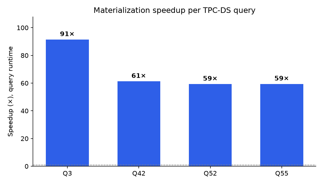
Creating a single materialization sped up the four queries between 59x and 91x, resulting in a 1.5x order of magnitude improvement in execution time. Also, we scan significantly less data (359GB vs. just 120MB) since the planner automatically rewrites our queries to scan the (much smaller) materialization instead. In this chart you can see the query runtime duration improvement of four TPC-DS queries (Q3, Q42, Q52 and Q55) after creating a single semantic view materialization.

Try it yourself

Materializations pay off when you have:

• Repeated AI agent or dashboard queries with similar patterns
• Additive metrics, so one fine-grained rollup can serve many coarser queries or similar, repeating query shapes
• Large base tables
• A staleness tolerance you can express with MAX_STALENESS.

The trade-off is straightforward: You spend background-refresh compute and some storage to speed up your repeated workloads.

Links

Docs:

• Materializing dimensions and metrics in semantic views
• Semantic views overview