

Summary
- Snowflake, the AI Data Cloud platform, was one of the first to launch support for Apache Iceberg™ v3. Support for Iceberg v3 Variant is generally available in Snowflake, with scans optimized for performance at production scale.
- Snowflake applies a decade of production-hardened Variant shredding to the open Parquet Variant Shredding spec — every shredded leaf becomes a real Parquet column with full columnar scan benefits, so projections and predicates push down to per-leaf columns.
- Snowflake completed an 11-query Iceberg v3 Variant benchmark in which it was 2.3x faster than Databricks on identical Iceberg tables at equivalent compute.
- Per-workload speedup benchmark results: 1.48x on field extraction, 9.47x on full-object retrieval, 3.37x on array element access and 1.78x on full-array retrieval.
The problem: Fast columnar scans on semi-structured data
Modern analytics fundamentally requires working with semi-structured data; this has not been an edge case for a long time. Previously, querying this data in an open format meant documents were treated as opaque blobs, forcing the engine to re-parse them at query time. This forced customers to choose between fast structured columns and flexible semi-structured formats. No portable open format could deliver both.
The Iceberg v3 Variant type bridges the gap between speed and flexibility. This is why it became our customers' most requested Iceberg v3 feature. While the Iceberg Variant type offers the theoretical framework, its real-world success depends on the underlying engine's sophisticated and efficient implementation.
Our approach: A decade of production experience, now in an open format
Snowflake has refined the Variant data type for over a decade, leveraging built-in shredding that automatically extracts fields into columnar subcolumns. This design, detailed in the SIGMOD 2016 paper, "The Snowflake Elastic Data Warehouse," enables metadata tracking and columnar optimizations for nested data.
With the ratification of the Iceberg v3 spec in June 2025 and the release of Parquet Variant Encoding and Shredding specs, Variant is now a first-class type in the open ecosystem. Industry adoption is growing, with third-party engines like DuckDB introducing native Variant support while crediting Snowflake as the inspiration.
Our implementation applies this extensive experience to the Parquet Variant Shredding spec, delivering the performance of native Snowflake tables within the open Iceberg ecosystem. Notably, Snowflake, the AI Data Cloud platform, was one of the first to launch general availability for Iceberg v3.
As Jacob Leverich, Co-Founder of Observe and Head of Technology, Observability at Snowflake, put: "Snowflake's long track record with Variant shredding at enterprise scale make it a no-brainer to power these solutions, now with Iceberg in the mix."
What we built: Iceberg Variant on Snowflake
Snowflake's Iceberg v3 Variant implementation enables full columnar efficiency for open tables. This feature is available on Iceberg v3 tables in Snowflake today, and customers benefit from columnar Variant scans without needing to adjust any other configurations. While Iceberg v3 Variant support is landing across the ecosystem, our system benefits from the same matured data-handling pattern we've run in production for a decade, ensuring our scan path is mature. We have also seen hundreds of customers use variant types during the preview period.
Principles for storing and retrieving semi-structured data
As the lakehouse model evolves to treat Variant as a first-class type, the scan layer must deliver on diverse performance requirements, without relying on format tricks that do not work on open formats, such as Parquet. At Snowflake, we follow clear guiding principles.
- Performance on nested data should "just work" without manual tuning or separate JSON paths. If you write SELECT payload:user.email FROM events, the engine should treat it like any other column projection.
- We optimize the write path. Data in a Variant column is shredded into columnar chunks at ingest, allowing the engine to bypass irrelevant paths. This upfront investment significantly reduces computational effort for all subsequent queries.
- We maintain open file formats. Everything occurs within standard Parquet files on object storage, using no proprietary sidecars or custom formats, ensuring full compatibility with other Iceberg engines that support the v3 standard.
How does Snowflake read Variant on Iceberg?
Variant shredding: Loading semi-structured data into a Variant column doesn't store documents as opaque blobs. Following the Variant Shredding spec, the engine shreds each document into a Parquet group of value / typed_value pairs at write time. A payload: {event_type, metrics: {timing: {load_ms}}} object is laid out as:
optional group payload (VARIANT(1)) {
  required binary metadata;         // shared Variant field-name dictionary
  optional binary value;            // Variant-encoded fallback for keys not in typed_value
  optional group typed_value {      // the shredded object
    required group event_type {     // simple shredded scalar
      optional binary value;        // fallback when a value isn't the shredded type
      optional binary typed_value (STRING);
    }
    required group metrics {        // nested object, shredded recursively
      optional binary value;
      optional group typed_value {
        required group timing {
          optional binary value;
          optional group typed_value {
            required group load_ms {
              optional binary value;
              optional int64 typed_value;
            }
          }
        }
      }
    }
  }
}
Nested objects (e.g., payload:metrics:timing:load_ms) shred recursively — each level becomes its own typed_value group, and the leaf becomes a typed Parquet column. Each shredded leaf is a real Parquet column with its own statistics (min/max, null count, distinct count). When a query runs SELECT payload:event_type::STRING FROM events against a fully shredded leaf, the engine scans the payload:typed_value:event_type.typed_value column chunk and bypasses the rest of the data entirely. No document reconstruction happens. No JSON parser runs at query time. Predicates like payload:event_type::STRING = 'purchase' push down to the per-leaf Parquet column, pruning unmatched data and making filtered aggregations faster.
Reassembly: The flip side of shredding is that whole-object and whole-array queries (Workload 2 and Workload 4 in our benchmark below) need to reconstruct the original Variant value from its shredded pieces. The Variant Shredding spec defines this assembly step precisely as a recursive walk of the typed_value group: at each shredded leaf the engine takes typed_value if present, otherwise falls back to the sibling value (for type-conflicting cases like a string stored where a timestamp was expected); and at the object root, the top-level value field is merged in to supply any keys not covered by the shredded schema (a "partially shredded object" in spec terms).
For queries that extract a specific field or array element (Workloads 1 and Workload 3 in our benchmark below) the engine never walks this path — it reads the shredded leaf and returns. For assembly queries it pays the reconstruction cost, but only on the columns the query actually projects, and the spec-defined layout means any Iceberg engine can reuse the same shredded files Snowflake produced.
Performance analysis and results
To evaluate variant column performance on Iceberg tables, we designed a simple benchmark comprising four workload categories that test the fundamental operations of storing and retrieving Variant data, the operations every semi-structured workload depends on. The benchmark data set is inspired by the open source Iceberg variant benchmark suite1, adapted to run on Snowflake-managed Iceberg tables.
The object workloads use an events_variant Iceberg table with 500M rows of synthetic event data containing a payload Variant column. The array workloads use an arrays_variant Iceberg table with 10M rows containing arrays of varying complexity (see Appendix for the table definition and data loading script). Both tables are stored as Iceberg tables with variant columns backed by the Iceberg Variant type specification.
Benchmark setup
Each query ran with two warmup runs followed by five measured runs.
The reported metric is the median end-to-end latency in milliseconds.
Snowflake queries ran on an XS Gen2 warehouse; Databricks queries ran on an XXS Serverless compute.
These two configurations are not architecturally identical — Snowflake and Databricks size and provision compute differently, so a direct comparison is not possible. The Snowflake XS Gen2 warehouse is a provisioned warehouse running on Snowflake's next-generation compute architecture; the Databricks XXS Serverless tier is a serverless SQL warehouse with a different sizing scheme and provisioning model. We selected the smallest production-grade tier each platform offers so that cost and scale stay in a comparable range, and we report wall-clock latency rather than per-credit or per-DBU efficiency to avoid mixing pricing assumptions into the result.
Headline results
Across all 11 queries on identical Iceberg tables, Snowflake completes the benchmark in 236 seconds vs. 553 seconds on Databricks when comparing on an equivalent compute — a 2.3x total wall-clock speedup (totals reflect the sum of median per-query runtimes across repeated executions). Per-workload median speedups:
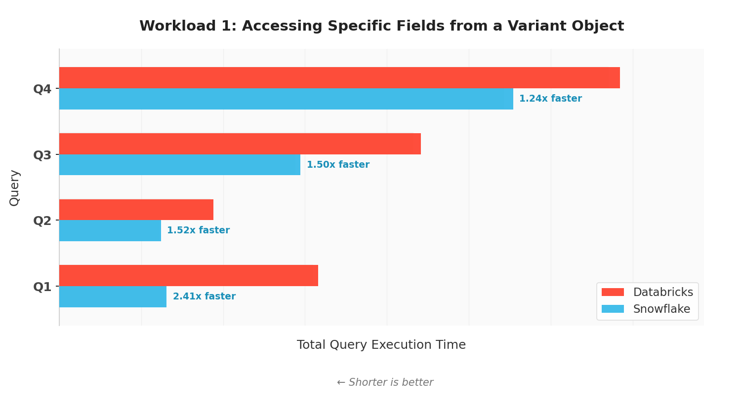
- Workload 1 — field extraction: 1.48x faster on Snowflake (Q1–Q4)
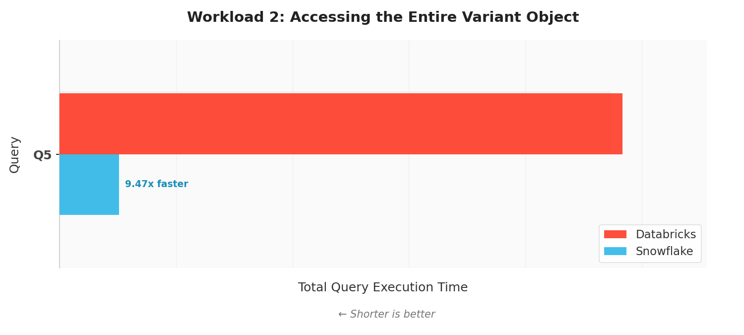
- Workload 2 — full-object retrieval: 9.47x faster on Snowflake (Q5)
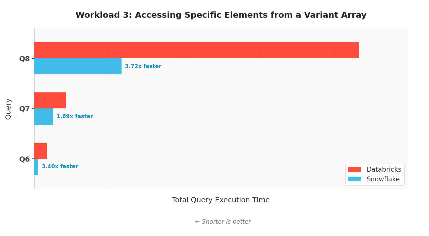
- Workload 3 — array element access: 3.37x faster on Snowflake (Q6–Q8)
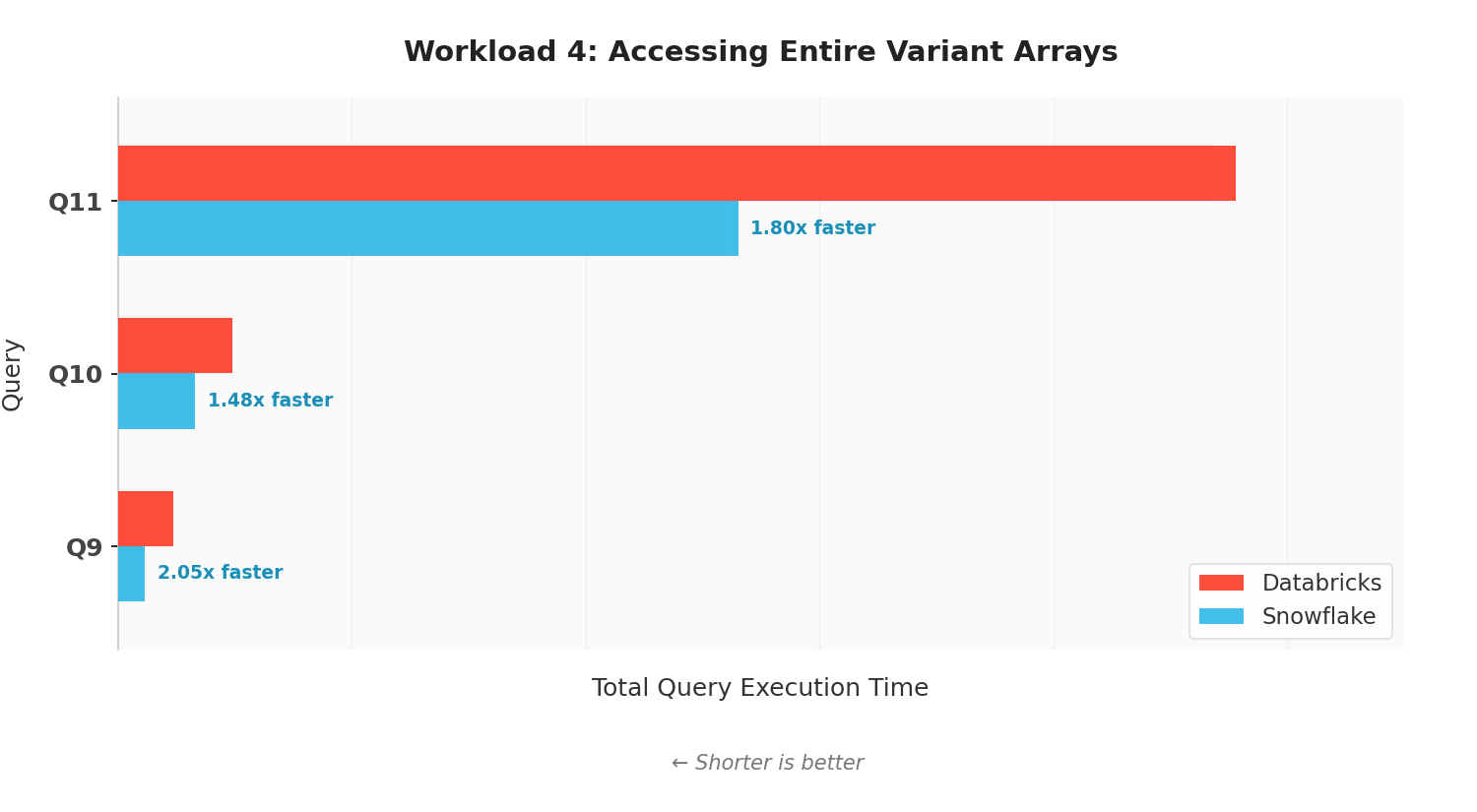
- Workload 4 — full-array retrieval: 1.78x faster on Snowflake (Q9–Q11)
Workload 1: Accessing specific fields from a Variant object
This workload targets point access into variant objects, extracting scalar fields by path. The queries progressively increase in complexity:
-- Q1: Top-level field aggregation
SELECT SUM(payload:duration::INT) FROM events_variant;

-- Q2: Deeply nested path traversal
SELECT SUM(payload:metrics.timing.load_ms::INT) FROM events_variant;

-- Q3: Filtered aggregation with predicates on variant fields
SELECT COUNT(event_id), SUM(payload:duration::INT)
FROM events_variant
WHERE payload:event_type::STRING = 'purchase'
  AND payload:country::STRING = 'US';

-- Q4: Grouped aggregation across variant fields
SELECT payload:event_type::STRING AS event_type,
       COUNT(event_id) AS cnt,
       SUM(payload:duration::INT) AS total_duration
FROM events_variant
GROUP BY payload:event_type::STRING;
These represent the most common operations on semi-structured data in analytical systems. Any platform ingesting semi-structured event data as JSON (clickstream tracking, application telemetry or transaction logs) relies heavily on these patterns. An analyst computing total session durations, filtering events by region for regional reporting, or breaking down metrics by event type for funnel analysis is executing exactly these query shapes.
In more complex pipelines, these operations are the inner building blocks. A monitoring system that detects anomalies will first extract nested timing fields (Q2-style), then apply filtered groupings (Q3/Q4-style) to segment by category and geography before feeding results into alerting logic. The engine's ability to push predicates into variant paths and prune data at the storage layer determines whether such pipelines remain interactive or degrade to batch.
Workload 2: Accessing the entire Variant object
This workload measures full-object retrieval, reading the complete variant payload, sorted by an extracted field:
-- Q5: Full object retrieval with sort
SELECT payload FROM events_variant ORDER BY payload:duration::INT LIMIT 10;
While field-level access dominates analytical queries, full-object retrieval is critical for debugging, data export and feeding downstream systems that need complete documents. An engineer investigating a failed transaction retrieves the full payload to inspect all fields. ETL pipelines that flatten variant data into structured tables must first read the entire object before applying transformations. The query uses ORDER BY with LIMIT to avoid result materialization cost and isolate the engine's ability to reconstruct complete objects from shredded variant data stored in Parquet.
Workload 3: Accessing specific elements from a Variant array
This workload tests positional element access on array-typed variant columns with increasing structural complexity:
-- Q6: Numeric element access
SELECT SUM(arr_number[0]::INT) FROM arrays_variant;

-- Q7: String element access
SELECT MIN(arr_text[0]::VARCHAR) FROM arrays_variant;

-- Q8: Nested 2D array element access
SELECT SUM(arr_graph[0][3]::INT) FROM arrays_variant;
The table stores arrays of 256 random strings, 256 random integers, and a 64x64 2D integer matrix per row, deliberately stressing the engine's ability to navigate variable-length structures.
Array positional access is common wherever entities carry multi-valued attributes. Embedding vectors stored as arrays require element-level access for similarity computations. Time-series sensor batches use positional indexing to retrieve readings at specific offsets. The nested 2D access (Q8) targets matrix-structured data like adjacency graphs or correlation matrices stored alongside analytical results. These element-level extractions form the inner loops of feature engineering and scientific computing pipelines where millions of lookups aggregate into derived metrics.
Workload 4: Accessing entire Variant arrays
The final workload combines full-array reconstruction with ordered access:
-- Q9: Full numeric array retrieval
SELECT arr_number FROM arrays_variant ORDER BY arr_number[0]::INT LIMIT 10;

-- Q10: Full string array retrieval
SELECT arr_text FROM arrays_variant ORDER BY arr_text[0]::VARCHAR LIMIT 10;

-- Q11: Full 2D array retrieval
SELECT arr_graph FROM arrays_variant ORDER BY arr_graph[0][3]::INT LIMIT 10;
Full-array retrieval is required when downstream consumers need the complete collection, exporting embedding vectors for model retraining, un-nesting arrays into normalized tables via FLATTEN or migrating data between schema versions. As with Workload 2, the queries use ORDER BY with LIMIT to avoid result materialization cost and focus purely on the engine's ability to reconstruct full variant arrays. The progressive complexity across numeric (Q9), string (Q10), and nested 2D (Q11) arrays reveals how each engine handles increasing payload size during full-structure reconstruction from shredded Parquet storage.
Summary
Iceberg v3 Variant moves semi-structured data from "the slow path" to a first-class columnar citizen, and Snowflake's implementation brings a decade of production-hardened shredding to that open contract. On the four workload categories that dominate real semi-structured analytics — field extraction, full-object retrieval, array element access and full-array retrieval — Snowflake completes the 11-query benchmark 2.3x faster than Databricks on identical Iceberg tables at equivalent compute.
We see this as the starting point, not the destination. Several improvements are already in active development, with more exciting work in the pipeline that we'll share in upcoming posts.
Appendix
The benchmark uses two Iceberg tables. The full table definitions, synthetic data-generation queries, and all 11 benchmark queries are available as two downloadable SQL files — one for each engine — so the benchmark can be rerun end-to-end against either:
- Snowflake: iceberg-variant-snowflake-all-queries.sql
- Databricks: iceberg-variant-databricks-all-queries.sql
Each file contains:
- Table definitions —
events_variant(500M rows; nested objects, arrays and scalar fields in a singlepayloadVariant column) andarrays_variant(10M rows; a 256-element string array, a 256-element integer array, and a 64×64 2D integer matrix as separate Variant columns). - Synthetic data-generation queries
- The 11 benchmark queries (Q1–Q11) cover all four workload categories: field extraction, full-object retrieval, array element access and full-array retrieval.
1Neelesh Salian


