Snowflake is investing in making it easier for AI agents to reason over business concepts and relationships natively. This blog shows what's possible today for teams with existing ontologies. Many industries maintain formal ontologies that provide an additional layer of domain-specific reasoning which can add to semantic reasoning captured over tables, columns and joins. This can help AI agents reason over hierarchy, synonymy and domain-specific concepts that a semantic layer alone may not fully capture.
Using a highly simplified biomedical data set, we compared a baseline semantic-view Cortex Agent with ontology-aware approaches built on knowledge graphs, GraphRAG and targeted terminology mappings. The results in this benchmark suggest that improved structural grounding may improve accuracy and reliability under the evaluated conditions, while also offering a practical blueprint for teams building enterprise AI agents that need to be more precise, explainable and trustworthy.
Incorporating Ontologies into Snowflake Cortex Agents
Enterprise data is full of meaning that never appears explicitly in a schema — inherent domain knowledge that must be captured to power reliable agentic systems.
Across industries, organizations maintain formal ontologies, taxonomies and controlled vocabularies to encode class hierarchies, typed relationships, constraints and canonical identifiers. In healthcare and life sciences, these include resources such as SNOMED CT, UMLS, the Gene Ontology and the Cell Ontology; in supply chain and retail, standards such as GS1 define product and packaging semantics; in financial services, FIBO provides a shared model for instruments, entities and regulatory classifications. These industry assets are typically published in representation formats such as OWL, RDF or SKOS and often contain thousands of concepts, rich synonym sets and tens of thousands of hierarchical and associative edges. Yet most enterprise AI and analytics systems still operate primarily over relational abstractions — tables, columns, keys and joins — without native access to the layers that define concept inheritance, transitive relationships, equivalence mappings or domain constraints. The result is a potential gap between how organizations model real-world meaning and how AI systems retrieve and reason over operational data.
Consider a supply chain analyst asking: "Show total spend across all electronic components," where "electronic component" sits atop a taxonomy of capacitors, resistors, ICs and dozens of subcategories. Or a biomedical researcher asking: "Show drug efficacy for PD-1 inhibitors across epithelial-derived cancer cell lines," which requires expanding a parent concept across dozens of cell types and 13 tissue categories. In both cases, Snowflake's semantic view provides the foundation of relational constructs (entities, relations, metrics, dimensions). In addition, the Recursive CTE (SQL extension) provides a dynamic path length query mechanism to support hierarchical typing and relationship axioms like subclass-of, transitive and inverse properties.
In this post, we look at what happens when you bring that deeper layer of ontological meaning into Snowflake and use it to ground AI agents alongside your operational data. Specifically, we evaluated a baseline semantic-layer approach and three ontology-aware enhancements on a biomedical benchmark designed to test ontology-dependent reasoning in agentic data retrieval tasks.
A biomedical benchmark
In drug discovery, finding new therapeutic candidates means navigating gene-pathway-cell-disease-drug-outcome relationships encoded in multiple ontologies disconnected from experimental data to derive insights. Our goal was to build and test agent architectures that can perform ontology-enabled reasoning, resolve semantic ambiguities and extract insights from cancer-cell line drug screening viability data (a measure of drug efficacy based on surviving cell ratio).
This benchmark is intended to show directional evidence. Its purpose was to measure incremental lift of ontology-aware techniques under controlled conditions by incorporating a single industry ontology for extracting insights in a complex data challenge. We combined two publicly available resources inside Snowflake:
- Cell ontology (CL): An ontology designed to classify and describe cell types encompassing 33,651 terms connected by ~50,000 hierarchical and relational edges.
- PRISM (Profiling Relative Inhibition Simultaneously in Mixtures) drug repurposing data set: Contains growth inhibitory activity of 4,518 drugs tested across 578 human cancer cell lines producing 2.6M+ viability measurements.
The bridging challenge is real: PRISM labels data by tissue (lung, breast), while the cell ontology organizes by lineage (epithelial cell, stromal cell). Agents must bridge this gap to answer analytical questions.
We wrote 22 hard questions intentionally targeted to isolate a specific problem: how an ontology-grounded agent performs in tasks spanning term resolution, cohort comparison, cross-tissue analysis, drug ranking, distribution analysis and multi-class comparison. Each agent tested ran five times to measure consistency.
Starting point: Semantic View, Agentic Analyst
Our baseline agent is leveraging semantic view, and uses Cortex Analyst, which translates natural language into validated SQL against that semantic layer.
Semantic view introduces a governed semantic layer above physical tables, allowing AI systems to work with a clear, domain-friendly model instead of raw schemas. Within a semantic view, we have entity tables, relations, facts, dimensions and metrics.
In the biomedical setting, that semantic layer can represent drugs, protein targets, cell lines and disease phenotypes as logical entities, use facts to capture measurable events such as drug-target interactions, use dimensions to provide analytic context such as tissue or disease state, and use metrics to encode derived measures such as potency or efficacy. This baseline provides a governed control point for measuring the incremental lift of ontology-aware techniques layered on top of the semantic model.
Our baseline agent serves as a control point to access the lift brought by other techniques.
Knowledge graph
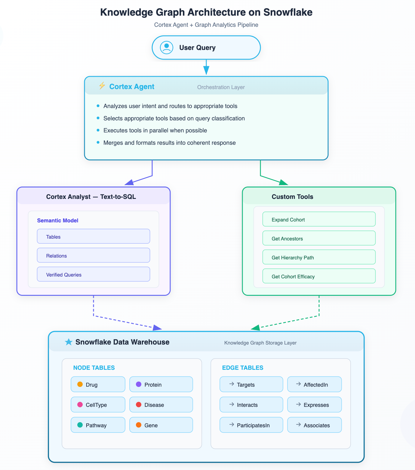
On top of the semantic view, we have implemented a simple knowledge graph using Snowflake tables to support graph traversal operation more naturally. A knowledge graph (KG), in this case, is a representation of knowledge as interconnected entities and typed relationships. (For a deeper dive on building knowledge graphs on Snowflake, see the Ontology on Snowflake blog series.)
Knowledge graph traversal
The knowledge graph is stored directly inside Snowflake using a node-edge table model:
- The KG_NODE table stores all entities, including their unique identifiers, type (drug, disease, cell) and properties (often stored in a flexible
VARIANTcolumn). - The KG_EDGE table stores relationships, including source node ID, target node ID, edge type (for example, treats, targets, expressed_in) and optional metadata, such as timestamps or confidence scores.
The implementation leverages Snowflake's distributed storage, automatic scaling, query optimization, security and governance without requiring a separate graph database.
Recursive CTE
A key capability of a knowledge graph is traversal — the ability to move from one entity to its connected neighbors across multiple hops, without knowing in advance how many steps are required. In Snowflake, this dynamic, variable-length traversal can be implemented using recursive common table expressions (CTEs). Recursive CTEs repeatedly join an edge table to itself, incrementally expanding the frontier of reachable nodes until no new nodes are found or a specified depth limit is reached or timeout. Unlike fixed self-joins, which require the number of hops to be hard-coded, recursive CTEs allow path length to remain data-driven and flexible.
Suppose we want to identify diseases mechanistically connected to a drug through biological pathways. The simplistic graph may contain edges, such as:
Drug →targets→ ProteinProtein →triggers→ PathwayPathway → expressed in → Cell TypeCell Type → affected in→ DiseaseDisease →subClassOf→ Disease Category(ontology hierarchy)
We may not know in advance whether a disease is reachable in two hops, three hops or via additional subclass expansions. A recursive CTE allows us to traverse this network dynamically.
On top of the baseline semantic view, the knowledge graph agent has additional access to four stored procedures (expand cohort, get ancestors, get hierarchy path, get cohort efficacy) plus two specialized Cortex Analyst semantic views, giving it seven tools total.
Example of such a tool:
  get_ancestors (GET_ANCESTORS_TOOL)
  Input: CONCEPT (e.g., "squamous epithelial cell")
  Data accessed: Ontology only -- KG_NODE + KG_EDGE
  Output: List of all ancestor nodes walking upward via subClassOf
    squamous epithelial cell
      → epithelial cell (depth 1)
        → eukaryotic cell (depth 2)
          → cell (depth 3)
            → anatomical structure (depth 4)
              → material anatomical entity (depth 5)
                → anatomical entity (depth 6)
  No PRISM data. Pure upward graph traversal.
Strength: Deterministic traversal across supported hierarchy depths. For "epithelial cell," this means all 693 descendants across 10+ hierarchy levels.
Weakness: Seven tools create orchestration complexity. The agent must choose the right tool sequence, and procedures require exact concept names with no synonym resolution.
Flattened GraphRAG
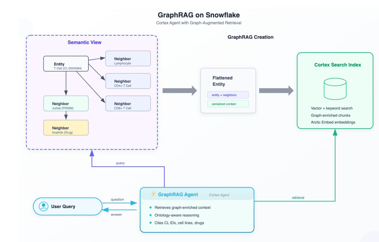
A complementary pattern is flattened GraphRAG. Instead of traversing an ontology or knowledge graph at query time, flattened GraphRAG precomputes a denormalized profile for each concept — combining its name, definition, synonyms, local neighborhood and attributes aggregated from descendants — and indexes those profiles in Cortex Search for hybrid keyword and vector retrieval.
At runtime, the agent retrieves the most relevant concept profile, extracts the grounded business or scientific context, and passes that context into Cortex Analyst or downstream SQL generation.
In Snowflake, the implementation pattern is straightforward: store the ontology in relational tables, use recursive CTEs or preprocessing pipelines to build one enriched profile per node, index those profiles with a Cortex Search service, and use the retrieved profile as the semantic grounding layer for analysis.
The advantage is a simpler retrieval architecture designed to improve consistency with strong synonym handling and no runtime graph traversal; the tradeoff is that the quality of the system depends heavily on how well the flattened profiles are constructed and refreshed.
Index construction
A preprocessing pipeline builds a neighborhood profile document for every ontology node. A recursive CTE traverses the full hierarchy (up to 15 levels via subClassOf edges), and for every node, collects descendant attributes and aggregates them upward. The result: Ancestor nodes contain aggregated tissue lists derived from their descendant trees.
Each document in the index contains:
- The node's formal name, definition and all known synonyms
- Immediate parents and children (first-order neighbors)
- Sample of grandparents and grandchildren (second-order neighbors)
- Aggregated domain data categories from all descendants
These profiles are indexed in a Cortex Search service with both keyword and vector embeddings.
On top of the baseline semantic view, the GraphRAG agent has just two tools: one search tool and one Cortex Analyst SQL tool. When a query arrives, the agent searches for the relevant entity profile, extracts the relevant categories and passes them explicitly to the SQL tool.
Strength: Synonym resolution via semantic search ("flat epithelial" resolves to "squamous epithelial cell"). Simpler two-tool architecture. No runtime graph traversal.
Weakness: Cannot resolve composite terms, such as "internal organ lining" that map to unions of multiple cell type categories. Requires periodic index rebuilds.
Adding terminology mapping instructions
Based on the GraphRAG agent, we enhanced the agent instructions by embedding hand-curated mappings directly in the agent's system prompt. For example, eight authoritative cell-type-to-tissue mappings and composite term definitions in our biomedical challenge act as overrides when they apply. For example, Squamous Epithelial Cell (CL:0000076) -> Skin, Lung, Esophagus, Bladder, Cervix hardcodes the relevant PRISM tissue mappings to any of the cell descendants in the cell ontology.
Strength: Eliminates the "last mile" error by collapsing multi-step lookups into a deterministic table.
Weakness: Static knowledge that must be manually maintained. Only covers mapped concepts; unmapped ones fall back to dynamic search.
Optimizing agents with Cortex Code
Building each agent configuration is only half the work. Tuning the system prompts, tool descriptions and selection heuristics to maximize accuracy is the other half. We used Cortex Code's agent optimization skills to iteratively refine all four agents. Cortex Code's optimization workflow made it straightforward to:
- Run the 22-question eval suite against each agent configuration
- Analyze failure patterns across runs
- Propose and apply prompt refinements (for example, the explicit tissue passthrough instruction for GraphRAG)
- Re-evaluate and compare results
This tight optimize-evaluate loop was critical. Several of the design choices that drove accuracy gains (search text enrichment with tissue keywords, the tissue passthrough mandate, shared statistical threshold rules) emerged directly from Cortex Code optimization iterations.
Results
The following table summarizes the findings from our benchmark evaluation.
| Agent Setup | Tool Count | Mean Score (/2.0) | Success Percentage |
|---|---|---|---|
| Standard Semantic View (Baseline) | 1 | 0.93 | 50.0% |
| Baseline with Knowledge Graph | 7 | 1.14 | 60.0% |
| Baseline with GraphRAG | 2 | 1.38 | 70.0% |
| Baseline with GraphRAG and Term Mappings | 2 | 1.55 | 78.2% |
Each enhancement showed improved benchmark performance within this evaluation framework. The knowledge graph approach produced an approximately 10 percentage point improvement in evaluated accuracy through exhaustive hierarchy expansion, while GraphRAG provided an additional approximate 10 percentage point improvement which may reflect the effects of simplified architecture and preintegrated descendant data. The terminology-mapping approach produced an additional improvement in evaluated accuracy within this benchmark by helping resolve complex domain aliases and composite terms.
Key Takeaway: In this benchmark, the observed improvements appeared to correlate more strongly with structural context than with increased computational reasoning.
Observations
1. Fix the data layer first. GraphRAG with aggregated descendant attributes captured a substantial portion of roughly 80% of the observed gain over baseline in this benchmark with no static mappings. Precomputing tissue lists appeared to be one of the most impactful interventions in this benchmark. Before investing in hand-curated rules, ensure the index provides complete data for every concept.
2. Fewer tools can also give good results. Within this benchmark, the flattened GraphRAG agent produced comparable results to the seven-tool knowledge graph agent. More tools give more raw capability but also more orchestration surface area for errors. GraphRAG's simplicity (one search tool, one SQL tool) reduces the agent's decision space and produces the lowest observed variance in this benchmark. Within this benchmark, the GraphRAG agent showed the lowest observed run-to-run variance, while the hardcoded-mapping variant, despite higher peak accuracy, showed the highest variance.
3. Targeted hardcoding closes the last gap. The terminology mapping agent's advantage over baseline GraphRAG configuration is concentrated on composite terms ("internal organ lining," "carcinoma-like models") that cannot be derived from hierarchy traversal alone. For a known, finite vocabulary of such terms, embedding curated mappings in the agent prompt is effective. This layer should stay thin: Supplement the index, do not replace it.
4. Cortex Code optimization skills make this workflow repeatable. Building an ontology-aware agent is an iterative process. Cortex Code's agent optimization skills provide the eval-refine-compare loop that turns architectural choices into measurable accuracy gains. The design decisions that mattered most in our results (search text enrichment, tissue passthrough, threshold rules) all emerged from this optimization process. Any team ingesting an ontology into Snowflake can follow the same workflow: Load the ontology; build the index; create an agent; and optimize with Cortex Code.
Biomedical nuance
This benchmark is best read as a comparative evaluation of ontology techniques, not as an attempt to maximize performance on the full scope of real-world biomedical reasoning. Our goal is not to claim coverage of the full biomedical reasoning stack, but to understand the relative contribution of different ontology-aware approaches under a simplified, controlled setting, and under what trade-offs in complexity, consistency and maintainability.
A production biomedical system would naturally extend beyond this setup. Real deployments often span multiple ontologies and multiple relation types at once, including cell types, anatomy, disease, pathway, compound identity, target biology and assay context. Over time, such systems should incorporate additional ontologies and controlled vocabularies, along with explicit provenance and uncertainty handling for each mapping step. But those are follow-on architecture concerns. The purpose of this benchmark is narrower: to compare ontology techniques on a simplified shared problem by looking at their relative performance.
Appendix A: Example of Recursive CTE
Here is an example of how recursive CTE can be used.
Natural language
Find all descendant cell types of EpithelialCell (follow subClassOf one or more hops), and return the full path(s) from EpithelialCell down to each descendant (For example, EpithelialCell → SquamousEpithelialCell → Keratinocyte).
SPARQL
PREFIX : <http://example.org/ontology/>
PREFIX rdfs: <http://www.w3.org/2000/01/rdf-schema#>

SELECT DISTINCT ?descendant
  WHERE {
    :EpithelialCell rdfs:subClassOf+ ?descendant .
  }
Recursive CTE
WITH RECURSIVE paths AS (
  -- anchor: direct children of the root 'EpithelialCell' (paths of length 1)
  SELECT
    e.src AS root,
    e.dst AS leaf,
    ARRAY[e.src, e.dst] AS path,
    1 AS depth
  FROM edges e
    WHERE e.src = 'EpithelialCell'

  UNION ALL

  -- recursive: extend existing paths by one child hop
  SELECT
    p.root,
    e.dst,
    p.path || e.dst AS path, -- append next node to path array
    p.depth + 1 AS depth
  FROM paths p JOIN edges e
    ON p.leaf = e.src
  WHERE NOT e.dst = ANY(p.path) -- avoid cycles
)

SELECT path, depth
FROM paths
  ORDER BY depth, path;