
This blog post presents a technique for automatically building database views based on the structure of JSON data stored in Snowflake tables. It’s a real time-saver, and you’ll find the complete code plus a usage example at the end of the second part of this blog post. Or, read on if you’d like to dig a little deeper, you’ll find details here on exactly how everything works!
Overview
One of Snowflake’s highly compelling features is its native support for semi-structured data. Of the supported file formats, JSON is one of the most widely used due to its relatively lightweight data-interchange format and the ease with which it can be written and read by both humans and machines. JSON data can be loaded directly into table columns of type VARIANT, and then queried using SQL SELECT statements that reference JSON document elements by their hierarchical paths. This requires some technical skills, however, along with knowledge about the JSON structure being queried. So, many organizations deploy views that essentially hide this complexity, thus making the data more easily accessible by end users. Creating and maintaining these views, however, is a manual process. These blog posts describe a technique that automates the creation of these views, which can help reduce errors and save time.
Background
Consider the following sample JSON data set:
{
  "ID": 1,
  "color": "black",
  "category": "hue",
  "type": "primary",
  "code": {
    "rgb": "255,255,255",
    "hex": "#000"
  }
},{
  "ID": 2,
  "color": "white",
  "category": "value",
  "code": {
    "rgb": "0,0,0",
    "hex": "#FFF"
  }
},{
  "ID": 3,
  "color": "red",
  "category": "hue",
  "type": "primary",
  "code": {
    "rgb": "255,0,0",
    "hex": "#FF0"
  }
},{
  "ID": 4,
  "color": "blue",
  "category": "hue",
  "type": "primary",
  "code": {
    "rgb": "0,0,255",
    "hex": "#00F"
  }
},{
  "ID": 5,
  "color": "yellow",
  "category": "hue",
  "type": "primary",
  "code": {
    "rgb": "255,255,0",
    "hex": "#FF0"
  }
},{
  "ID": 6,
  "color": "green",
  "category": "hue",
  "type": "secondary",
  "code": {
    "rgb": "0,255,0",
    "hex": "#0F0"
  }
}
Although JSON data is typically bulk loaded into a destination table using a COPY INTO operation, the above data set is sufficiently small that it can be loaded into a Snowflake table using a CREATE TABLE AS (CTAS) command, like so:
CREATE OR REPLACE TABLE colors AS
SELECT
   parse_json(column1) AS json_data
FROM VALUES
   ('{
      "ID": 1,
      "color": "black",
      "category": "hue",
      "type": "primary",
      "code": {
        "rgb": "255,255,255",
        "hex": "#000"
      }
    }'),
   ('{
      "ID": 2,
      "color": "white",
      "category": "value",
      "code": {
        "rgb": "0,0,0",
        "hex": "#FFF"
      }
    }'),
   ('{
      "ID": 3,
      "color": "red",
      "category": "hue",
      "type": "primary",
      "code": {
        "rgb": "255,0,0",
        "hex": "#FF0"
      }
    }'),
   ('{
      "ID": 4,
      "color": "blue",
      "category": "hue",
      "type": "primary",
      "code": {
        "rgb": "0,0,255",
        "hex": "#00F"
      }
    }'),
   ('{
      "ID": 5,
      "color": "yellow",
      "category": "hue",
      "type": "primary",
      "code": {
        "rgb": "255,255,0",
        "hex": "#FF0"
      }
    }'),
   ('{
      "ID": 6,
      "color": "green",
      "category": "hue",
      "type": "secondary",
      "code": {
        "rgb": "0,255,0",
        "hex": "#0F0"
      }
    }')
    as raw_json;
Here’s how this data can be queried:
SELECT
    json_data:ID::INTEGER as ID,
    json_data:color::STRING as color,
    json_data:category::STRING as category,
    json_data:type::STRING as type,
    json_data:code.rgb::STRING as code_rgb,
    json_data:code.hex::STRING as code_hex
FROM
    colors;
+----+--------+----------+-----------+-------------+----------+
| ID | COLOR  | CATEGORY | TYPE      | CODE_RGB    | CODE_HEX |
|----+--------+----------+-----------+-------------+----------|
|  1 | black  | hue      | primary   | 255,255,255 | #000     |
|  2 | white  | value    | NULL      | 0,0,0       | #FFF     |
|  3 | red    | hue      | primary   | 255,0,0     | #FF0     |
|  4 | blue   | hue      | primary   | 0,0,255     | #00F     |
|  5 | yellow | hue      | primary   | 255,255,0   | #FF0     |
|  6 | green  | hue      | secondary | 0,255,0     | #0F0     |
+----+--------+----------+-----------+-------------+----------+
Note the references to the JSON document elements by their hierarchical paths, for example:
json_data:code.rgb::STRING as code_rgb
Where:
- json_data: Specifies the VARIANT column in which the JSON data resides
- code.rgb: Is the path to the RGB element in the JSON document structure
- STRING: Casts the data to the appropriate type
- code_rgb: Is the alias for the corresponding column in the result set
A view could manually be created that essentially hides this complexity from the end user community, such as:
CREATE OR REPLACE VIEW
    colors_vw
AS SELECT
    json_data:ID::INTEGER as ID,
    json_data:color::STRING as color,
    json_data:category::STRING as category,
    json_data:type::STRING as type,
    json_data:code.rgb::STRING as code_rgb,
    json_data:code.hex::STRING as code_hex
FROM
    colors;
The problem here is that someone has to manually create that view. And that view would need to be updated if additional elements are added to the underlying JSON, hence the desire to automate this process!
View Creation Steps
To automate the creation of such a view, we’ll need to know two key pieces of information about each element in the JSON document structure:
- The paths to each element
- The data type of each element
It turns out that we can leverage a LATERAL join to a FLATTEN subquery to get information about the individual elements in the JSON document structure, like so:
SELECT DISTINCT
   f.path,
   typeof(f.value)
FROM
  colors,
  LATERAL FLATTEN(json_data, RECURSIVE=>true) f
WHERE
  TYPEOF(f.value) != 'OBJECT';
+----------+-----------------+
| PATH     | TYPEOF(F.VALUE) |
|----------+-----------------|
| ID       | INTEGER         |
| category | VARCHAR         |
| code.hex | VARCHAR         |
| code.rgb | VARCHAR         |
| type     | VARCHAR         |
| color    | VARCHAR         |
+----------+-----------------+
Now that we know how to get this information, we’ll need a programmatic mechanism that allows us to actually automate the view creation process. Here’s what it’ll need to do:
- Build the query that returns the elements and their data types
- Run the query
- Loop through the returned elements
- Build the view column list
- Construct the view Data Definition Language (DDL):
CREATE VIEW … AS SELECT … - Run the DDL to create the view
It turns out that Snowflake’s JavasScript stored procedures are perfect for this use case.
Stored Procedure Components
The stored procedure that we’ll build will accept three parameters:
- TABLE_NAME: The name of the table that contains the semi-structured data.
- COL_NAME: The name of the VARIANT column in the aforementioned table.
- VIEW_NAME: The name of the view to be created by the stored procedure.
Here’s what the shell of our stored procedure will look like:
create or replace procedure create_view_over_json
   (TABLE_NAME varchar, COL_NAME varchar, VIEW_NAME varchar)
returns varchar
language javascript
as
$
Build the view…
$;
Let’s look at each of the steps outlined earlier, along with the corresponding stored procedure code.
1. Build the Query that Returns the Elements and Their Data tTypes
The variable element_query will contain the text of the query:
var element_query = "SELECT DISTINCT n" +
                    path_name + " AS path_name, n" +
                    attribute_type + " AS attribute_type, n" +
                    alias_name + " AS alias_name n" +
                    "FROM n" +
                    TABLE_NAME + ", n" +
                    "LATERAL FLATTEN(" + COL_NAME + ", RECURSIVE=>true) f n" +
                    "WHERE TYPEOF(f.value) != 'OBJECT' n";
Note the references to the TABLE_NAME and COL_NAME parameters.
Definitions of the path name, attribute type, and alias name have been broken out from this query definition to make it easier to read. Here’s how each of these are defined:
- Path name: This generates paths with levels enclosed by double quotes (example: “path”.”to”.”element”):
var path_name = “regexp_replace(f.path,'(\\w+)’,'”\\1″‘)”;
Note the doubled-up instances of the ” escape character; – this has to be done because since there are two interpreters involved in the execution of the statement (JavasScript and SQL). - Attribute type: This generates column data types of ARRAY, BOOLEAN, FLOAT, and STRING only:
var attribute_type = “DECODE (substr(typeof(f.value),1,1),’A’,’ARRAY’,’B’,’BOOLEAN’,’I’,’FLOAT’,’D’,’FLOAT’,’STRING’)”;
This helps ensure the DISTINCT clause of the SELECT works properly, which – this prevents cases where the same element is returned with multiple data types (eg. INTEGER and FLOAT, for example). We’ll discuss this in more detail in the second blog post. - Alias: This generates column aliases based on the path:
var alias_name = “REGEXP_REPLACE(REGEXP_REPLACE(f.path, ‘\\[(.+)\\]’),'[^a-zA-Z0-9]’,’_’)” ;
It’s important to note that the query will return these three values for each element in the JSON document structure.
2. Run the Query
This is pretty straightforward. First, the text of the query contained inby element_query is used to create an executable statement object using the createStatement() method:
var element_stmt = snowflake.createStatement({sqlText:element_query});
Next, the statement object is executed using the execute() method:
var element_res = element_stmt.execute();
Note that the query result set is returned as the element_res object.
3. Loop Through the Returned Elements
The goal here is to build column expressions that look like this: col_name:”name”.”first”::STRING as name_first
This is done by looping through the query result set using the next() method and building out the desired column expression using the path:
while (element_res.next()) {
      col_list += COL_NAME + ":" + element_res.getColumnValue(1);   // Path name
      col_list += "::" + element_res.getColumnValue(2);             // Datatype
      col_list += " as " + element_res.getColumnValue(3);           // Alias
     }
Note that the COL_NAME parameter is used again here as part of the column expression build.
4. Build the View Column List
It turns out that the column list was being built as we looped through the query result set. We did that through a series of appends to the col_list string (the += operator does this in the code shown in the section above).
5. Construct the View DDL
Now that we’ve got the column list, we can simply “splice” it into the view DDL string, like so:
var view_ddl = "CREATE OR REPLACE VIEW " + VIEW_NAME + " AS n" +
               "SELECT n" + col_list + "n" +
               "FROM " + TABLE_NAME;
6. Run the DDL to Create the View
Even though this is a DDL statement, we’ll use the same createStatement() and execute() methods as we used when we ran the element list query (step 2, above):
var view_stmt = snowflake.createStatement({sqlText:view_ddl});
var view_res = view_stmt.execute();
Putting It All Together
Now that we’ve got all the pieces we need, we’re ready to create the stored procedure. Here’s the complete code:
create or replace procedure create_view_over_json (TABLE_NAME varchar, COL_NAME varchar, VIEW_NAME varchar)
returns varchar
language javascript
as
$
// CREATE_VIEW_OVER_JSON - Craig Warman, Snowflake Computing, DEC 2019
//
// This stored procedure creates a view on a table that contains JSON data in a column.
// of type VARIANT.  It can be used for easily generating views that enable access to
// this data for BI tools without the need for manual view creation based on the underlying
// JSON document structure.
//
// Parameters:
// TABLE_NAME    - Name of table that contains the semi-structured data.
// COL_NAME      - Name of VARIANT column in the aforementioned table.
// VIEW_NAME     - Name of view to be created by this stored procedure.
//
// Usage Example:
// call create_view_over_json('db.schema.semistruct_data', 'variant_col', 'db.schema.semistruct_data_vw');
//
// Important notes:
//   - This is the "basic" version of a more sophisticated procedure. Its primary purpose
//     is to illustrate the view generation concept.
//   - This version of the procedure does not support:
//         - Column case preservation (all view column names will be case-insensitive).
//         - JSON document attributes that are SQL reserved words (like TYPE or NUMBER).
//         - "Exploding" arrays into separate view columns - instead, arrays are simply
//           materialized as view columns of type ARRAY.
//   - Execution of this procedure may take an extended period of time for very
//     large datasets, or for datasets with a wide variety of document attributes
//     (since the view will have a large number of columns).
//
// Attribution:
// I leveraged code developed by Alan Eldridge as the basis for this stored procedure.

var path_name = "regexp_replace(regexp_replace(f.path,'\\\\[(.+)\\\\]'),'(\\\\w+)','"\\\\1\"')"                           // This generates paths with levels enclosed by double quotes (ex: "path"."to"."element").  It also strips any bracket-enclosed array element references (like "[0]")
var attribute_type = "DECODE (substr(typeof(f.value),1,1),'A','ARRAY','B','BOOLEAN','I','FLOAT','D','FLOAT','STRING')";    // This generates column datatypes of ARRAY, BOOLEAN, FLOAT, and STRING only
var alias_name = "REGEXP_REPLACE(REGEXP_REPLACE(f.path, '\\\\[(.+)\\\\]'),'[^a-zA-Z0-9]','_')" ;                           // This generates column aliases based on the path
var col_list = "";

// Build a query that returns a list of elements which will be used to build the column list for the CREATE VIEW statement
var element_query = "SELECT DISTINCT \n" +
                    path_name + " AS path_name, \n" +
                    attribute_type + " AS attribute_type, \n" +
                    alias_name + " AS alias_name \n" +
                    "FROM \n" +
                    TABLE_NAME + ", \n" +
                    "LATERAL FLATTEN(" + COL_NAME + ", RECURSIVE=>true) f \n" +
                    "WHERE TYPEOF(f.value) != 'OBJECT' \n" +
                    "AND NOT contains(f.path,'[') ";      // This prevents traversal down into arrays;

// Run the query...
var element_stmt = snowflake.createStatement({sqlText:element_query});
var element_res = element_stmt.execute();

// ...And loop through the list that was returned
while (element_res.next()) {

// Add elements and datatypes to the column list
// They will look something like this when added:
//    col_name:"name"."first"::STRING as name_first,
//    col_name:"name"."last"::STRING as name_last

   if (col_list != "") {
      col_list += ", \n";}
   col_list += COL_NAME + ":" + element_res.getColumnValue(1);   // Start with the element path name
   col_list += "::" + element_res.getColumnValue(2);             // Add the datatype
   col_list += " as " + element_res.getColumnValue(3);           // And finally the element alias
}

// Now build the CREATE VIEW statement
var view_ddl = "CREATE OR REPLACE VIEW " + VIEW_NAME + " AS \n" +
               "SELECT \n" + col_list + "n\" +
               "FROM " + TABLE_NAME;

// Now run the CREATE VIEW statement
var view_stmt = snowflake.createStatement({sqlText:view_ddl});
var view_res = view_stmt.execute();
return view_res.next();
$;
Here’s how it would be run against the COLORS table that was created earlier:
call create_view_over_json('mydatabase.public.colors', 'json_data', 'mydatabase.public.colors_vw');
Note the three parameters mentioned earlier:
- TABLE_NAME: The name of the table that contains the semi-structured data (mydatabase.public.colors).
- COL_NAME: The name of the VARIANT column in the aforementioned table (json_data).
- VIEW_NAME: The name of the view to be created by the stored procedure (mydatabase.public.colors_vw).
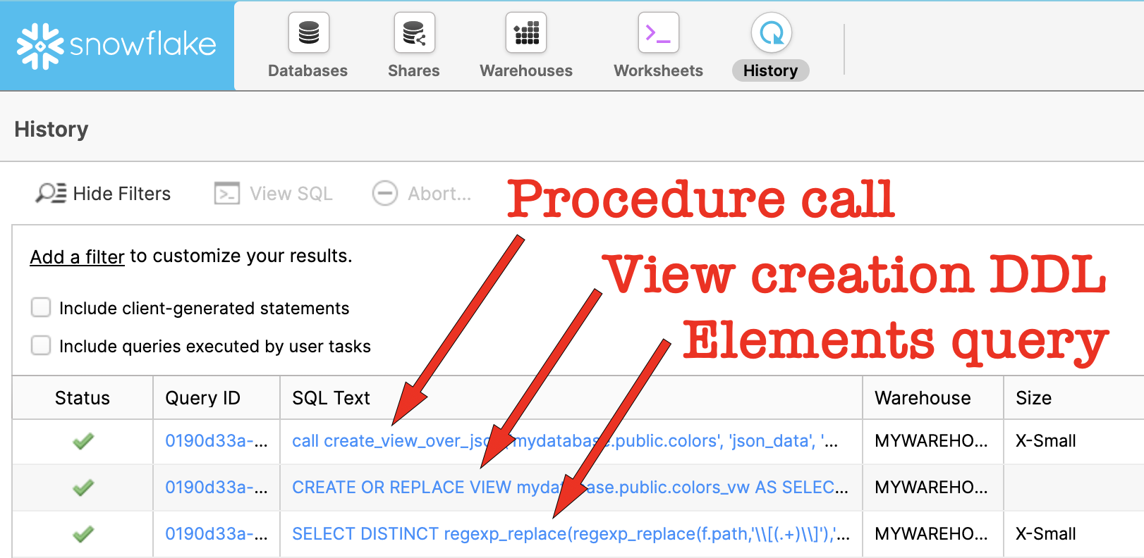
If you execute the code above and then look at the History tab, you’ll see three SQL statements being executed. First, you’ll see the stored procedure call, and then beneath that you’ll see where it ran the query that returns the elements and their data types; and then you’ll see where it executed the view creation DDL:
Click the DDL generated by the stored procedure. It should look something like this:
CREATE OR REPLACE VIEW mydatabase.public.colors_vw AS
SELECT
json_data:"ID"::FLOAT as ID,
json_data:"category"::STRING as category,
json_data:"code"."hex"::STRING as code_hex,
json_data:"code"."rgb"::STRING as code_rgb,
json_data:"color"::STRING as color,
json_data:"type"::STRING as type
FROM mydatabase.public.colors
Here’s the view description:
desc view colors_vw;
+----------+-------------------+--------+-------+---------+-------------+------------+-------+------------+---------+
| name     | type              | kind   | null? | default | primary key | unique key | check | expression | comment |
|----------+-------------------+--------+-------+---------+-------------+------------+-------+------------+---------|
| ID       | FLOAT             | COLUMN | Y     | NULL    | N           | N          | NULL  | NULL       | NULL    |
| CATEGORY | VARCHAR(16777216) | COLUMN | Y     | NULL    | N           | N          | NULL  | NULL       | NULL    |
| CODE_HEX | VARCHAR(16777216) | COLUMN | Y     | NULL    | N           | N          | NULL  | NULL       | NULL    |
| CODE_RGB | VARCHAR(16777216) | COLUMN | Y     | NULL    | N           | N          | NULL  | NULL       | NULL    |
| COLOR    | VARCHAR(16777216) | COLUMN | Y     | NULL    | N           | N          | NULL  | NULL       | NULL    |
| TYPE     | VARCHAR(16777216) | COLUMN | Y     | NULL    | N           | N          | NULL  | NULL       | NULL    |
+----------+-------------------+--------+-------+---------+-------------+------------+-------+------------+---------+
And, finally, here’s what the resulting data set looks like:
select * from colors_vw;
+----+----------+----------+-------------+--------+-----------+
| ID | CATEGORY | CODE_HEX | CODE_RGB    | COLOR  | TYPE      |
|----+----------+----------+-------------+--------+-----------|
|  1 | hue      | #000     | 255,255,255 | black  | primary   |
|  2 | value    | #FFF     | 0,0,0       | white  | NULL      |
|  3 | hue      | #FF0     | 255,0,0     | red    | primary   |
|  4 | hue      | #00F     | 0,0,255     | blue   | primary   |
|  5 | hue      | #FF0     | 255,255,0   | yellow | primary   |
|  6 | hue      | #0F0     | 0,255,0     | green  | secondary |
+----+----------+----------+-------------+--------+-----------+
It’s a whole lot easier to execute that one stored procedure call than to manually create the view!
What’s Next?
A lot, actually. This stored procedure was actually pretty basic in its construction; – its primary purpose is to illustrate the concept of how the overall process essentially works. Before we consider using this stored procedure on a regular basis, there are some things that need to be considered:
- Column case: Should the generated view’s column case match that of the JSON elements, or should all of the columns just be capitalized? At this point, the stored procedure simply creates all of the view columns as uppercase, which is Snowflake’s default behavior.
- Column types: Right now we’re setting the data type of each view column so that it matches that of the underlying data. But, sometimes there are cases where multiple JSON documents have attributes with the same name but actually contain data with different data types, and this can lead to problems.
- Arrays: JSON documents can contain both simple and object arrays, and the current stored procedure simply returns these as view columns of data type ARRAY. It would be desirable to have the contents of these arrays exposed as separate view columns.
We’ll tackle each of these in the second part of this blog post!