Getting Started with Snowflake Interactive Tables
Overview
When it comes to near real-time (or sub-second) analytics, the ideal scenario involves achieving consistent, rapid query performance and managing costs effectively, even with large datasets and high user demand.
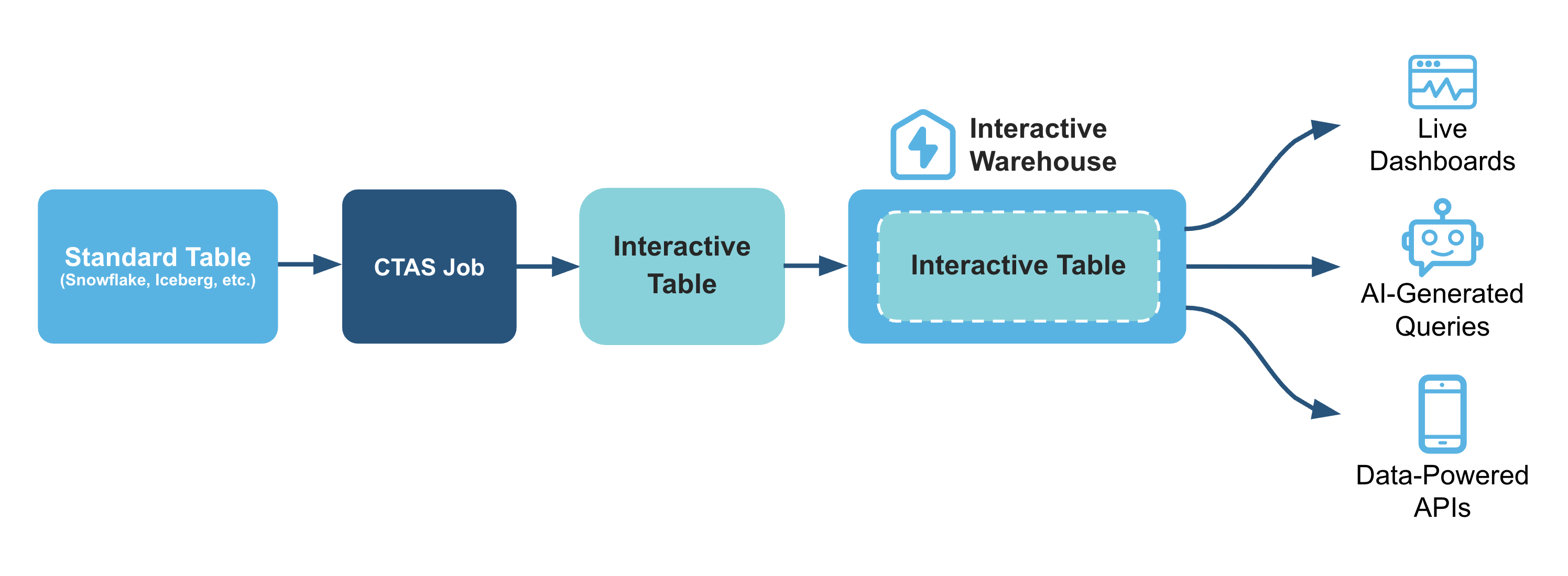
Snowflake's new Interactive Warehouses and Tables are designed to deliver on these needs. They provide high-concurrency, low-latency serving layer for near real-time analytics. This allows consistent, sub-second query performance for live dashboards and APIs with great price-for-performance. With this end-to-end solution, you can avoid operational complexities and tool sprawl.
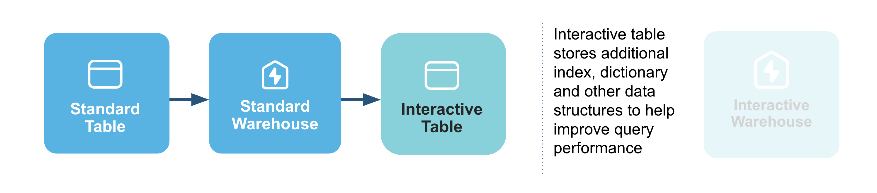
Here's how interactive warehouses and tables fits in for a typical data analytics pipeline:
What You'll Learn
- The core concepts behind Snowflake's Interactive Warehouses and Tables and how they provide low-latency analytics.
- How to create and configure an Interactive Warehouse using SQL.
- The process of creating an Interactive Table from an existing standard table.
- How to attach a table to an Interactive Warehouse to pre-warm the data cache for faster queries.
- A methodology for benchmarking and comparing the query latency of an interactive setup versus a standard warehouse.
What You'll Build
You will build a complete, functioning interactive data environment in Snowflake, including a dedicated Interactive Warehouse and an Interactive Table populated with data. You will also create a Python-based performance test that executes queries against both your new interactive setup and a standard configuration, culminating in a comparative bar chart that visually proves the latency improvements.
Prerequisites
- Access to a Snowflake account
- Basic knowledge of SQL and Python.
- Familiarity with data warehousing and performance concepts.
- A Snowflake role with privileges to create warehouses and tables (i.e.,
SYSADMINis used in the notebook).
Understand Interactive Warehouses and Interactive Tables
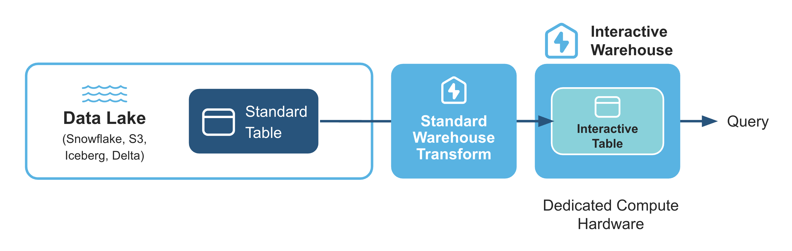
To boost query performance for interactive, sub-second analytics, Snowflake introduces two new, specialized objects that work together: interactive warehouses and interactive tables.
Think of them as a high-performance pair. Interactive tables are structured for extremely fast data retrieval, and interactive warehouses are the specialized engines required to query them. Using them in tandem is the key to achieving the best possible query performance and lowest latency.
Interactive Warehouses
An interactive warehouse tunes the Snowflake engine specially for low-latency, interactive workloads. This type of warehouse is optimized to run continuously, serving high volumes of concurrent queries. All interactive warehouses run on the latest generation of hardware and can only query interactive tables.
Interactive Tables
Interactive tables have different methods for data ingestion and support a more limited set of SQL statements and query operators than standard Snowflake tables.
Use cases
Snowflake interactive tables are optimized for fast, simple queries when you require consistent low-latency responses. Interactive warehouses provide the compute resources required to serve these queries efficiently. Together, they enable use cases such as live dashboards, data-powered APIs, and serving high-concurrency workloads.
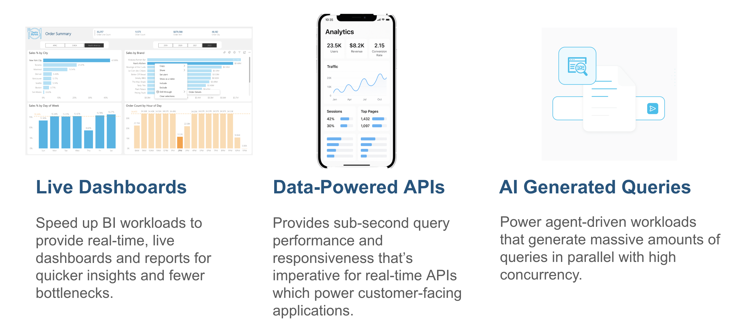
Furthermore, this pairing of interactive warehouses and tables is ideal for a range of specific, demanding use cases where sub-second query performance is paramount. In industries like ad-tech, IoT, and video analytics, it can power near real-time decisioning on massive event streams. For application development, it enables highly responsive data-powered APIs and in-app user behavior analytics. It's also perfectly suited for internal analytics, providing the speed needed for live dashboards, BI acceleration, and critical observability/APM systems that require high-throughput alerting.
Limitations
The queries that work best with interactive tables are usually SELECT statements with selective WHERE clauses, optionally including a GROUP BY clause on a few dimensions.
Here are some limitations of interactive warehouses and interactive tables:
- An interactive warehouse is always up and running by design. You can manually suspend the warehouse, but expect significant query latency when you resume the warehouse.
- Snowflake interactive tables don't support ETL, long-running queries (more than 5 seconds), or data manipulation language (DML) commands such as
UPDATEandDELETE. - Do modify data, you should update the data in source tables and either fully replace an interative table with new version, or use a dynamic table style incremental refresh by setting TARGET_LAG
- You can't query standard Snowflake tables from an interactive warehouse. To query both standard tables and interactive tables in the same session, run
USE WAREHOUSEto switch to the appropriate warehouse type depending on the type of table. - You can't run
CALLcommands to call stored procedures through interactive warehouse
Setup
Data operations
Optional: Create warehouse
In order to create an interactive table and fill the table with data, you'll need to use a standard warehouse.
You can use any existing warehouse or create a new one, here we'll create a new warehouse called WH:
CREATE OR REPLACE WAREHOUSE WH WITH WAREHOUSE_SIZE='X-SMALL';
Step 1: Create a Database and Schema
First, we'll start by creating a database called MY_DEMO_DB and BENCHMARK_FDN and BENCHMARK_INTERACTIVE as schemas:
CREATE DATABASE IF NOT EXISTS MY_DEMO_DB;
CREATE SCHEMA IF NOT EXISTS MY_DEMO_DB.BENCHMARK_FDN;
CREATE SCHEMA IF NOT EXISTS MY_DEMO_DB.BENCHMARK_INTERACTIVE;
Step 2: Create a new stage
Next, we'll create a stage called my_csv_stage where the CSV file will soon be stored:
-- Define database and schema to use
USE SCHEMA MY_DEMO_DB.BENCHMARK_FDN;

-- Create a stage that includes the definition for the CSV file format
CREATE OR REPLACE STAGE my_csv_stage
  FILE_FORMAT = (
    TYPE = 'CSV'
    SKIP_HEADER = 1
    FIELD_OPTIONALLY_ENCLOSED_BY = '"'
  );
Step 3: Upload CSV to a stage
- In the Snowflake UI, navigate to the database/schema that you've created (
MY_DEMO_DB.BENCHMARK_FDN). - Go to the
my_csv_stagestage - Upload the
synthetic_hits_data.csvfile to this stage.
Step 4: Create the Table and Load Data
Now that we have the CSV file in the stage, we'll need to create the HITS2_CSV table and extract contents from the CSV file into it.
-- Use your database and schema
USE SCHEMA MY_DEMO_DB.BENCHMARK_FDN;

-- Create the table with the correct data types
CREATE OR REPLACE TABLE HITS2_CSV (
    EventDate DATE,
    CounterID INT,
    ClientIP STRING,
    SearchEngineID INT,
    SearchPhrase STRING,
    ResolutionWidth INT,
    Title STRING,
    IsRefresh INT,
    DontCountHits INT
);

-- Copy the data from your stage into the table
-- Make sure to replace 'my_csv_stage' with your stage name
COPY INTO HITS2_CSV FROM @my_csv_stage/synthetic_hits_data.csv
  FILE_FORMAT = (TYPE = 'CSV' SKIP_HEADER = 1);
Step 5: Query the data
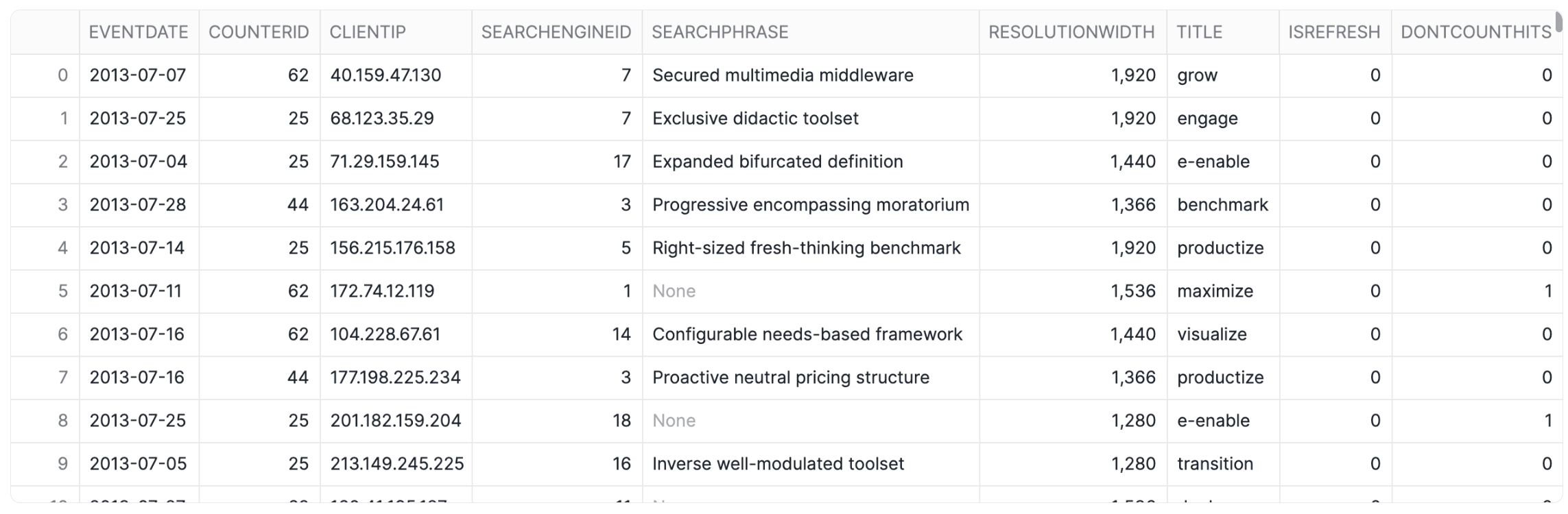
Finally, we'll now retrieve contents from the table by performing a simple query with the SELECT statement:
-- Query
SELECT * FROM MY_DEMO_DB.BENCHMARK_FDN.HITS2_CSV;
This essentially retrieves data from the MY_DEMO_DB database, BENCHMARK_FDN schema and HITS2_CSV table:
Performance Demo of Snowflake's Interactive Warehouses/Tables
To proceed with carrying out this performance comparison of interactive warehouses/tables with standard ones, you can download notebook file Getting_Started_with_Interactive_Tables.ipynb provided in the repo.
Load libraries and define custom functions
We'll start by loading the prerequisite libraries and define helper functions that will be used for the benchmark.
import snowflake.connector as snow
import matplotlib.pyplot as plt
import numpy as np
import pandas as pd
import time
import datetime
import random
import statistics
import tabulate
from concurrent.futures import ThreadPoolExecutor, as_completed

from snowflake.snowpark.context import get_active_session
session = get_active_session()
conn_kwargs = {"connection": session.connection}

def execute_and_print(query):
    cursor.execute(query)
    print(tabulate.tabulate(cursor.fetchall()))

def run_and_measure(count, mode):
    if mode == "std":
        query = """
                SELECT SearchEngineID, ClientIP, COUNT(*) AS c, SUM(IsRefresh), AVG(ResolutionWidth) FROM
                BENCHMARK_FDN.HITS2_CSV
                WHERE SearchPhrase <> '' GROUP BY SearchEngineID, ClientIP ORDER BY c DESC LIMIT 10;
                """
        cursor.execute("USE WAREHOUSE wh")
    else:
        query = """
                SELECT SearchEngineID, ClientIP, COUNT(*) AS c, SUM(IsRefresh), AVG(ResolutionWidth) FROM
                BENCHMARK_INTERACTIVE.CUSTOMERS
                WHERE SearchPhrase <> '' GROUP BY SearchEngineID, ClientIP ORDER BY c DESC LIMIT 10;
                """
        cursor.execute("USE WAREHOUSE interactive_demo_b")

    timings = []
    cursor.execute('ALTER SESSION SET USE_CACHED_RESULT = FALSE;')
    for i in range(count + 1):
        t0 = time.time()
        cursor.execute(query).fetchall()
        time_taken = time.time() - t0
        timings.append(time_taken)

    return timings[1:]

def plot_data(data, title, time_taken, color='#29B5E8'):
    # Separate titles and counts
    titles = [item[0] for item in data]
    counts = [item[1] for item in data]

    # Plot bar chart

    plt.figure(figsize=(12, 4))
    plt.bar(titles, counts, color=color)
    plt.xticks(rotation=45, ha='right')
    plt.ylabel("Counts")
    plt.xlabel("Title")
    plt.title(title)
    plt.text(0.5, 1.5, f'Time taken: {time_taken:.4f} seconds',
         ha='center', va='top',
         transform=plt.gca().transAxes,
         fontdict={'size': 16})
    #plt.tight_layout()
    plt.show()
Setting up connection to a Snowflake deployment and verifying versions
Here, we'll connect to Snowflake and verify the version and confirm that key interactive features are enabled, before setting the active database and role for the session.
cursor = session.connection.cursor()

execute_and_print('select current_version();')
execute_and_print("show parameters like 'ENABLE_INTERACTIVE_WAREHOUSES' for account;")
execute_and_print("show parameters like 'ENABLE_INTERACTIVE_TABLE_DDL' for account;")
execute_and_print("show parameters like 'SHOW_INCLUDE_INTERACTIVE_TABLES' for account;")

query = """ USE DATABASE MY_DEMO_DB;
"""
execute_and_print(query)

query = """ USE ROLE SYSADMIN;
"""
execute_and_print(query)
Create an interactive warehouse

Next, let's create our interactive_demo_b warehouse and immediately turn it on:
query = """
CREATE or REPLACE INTERACTIVE WAREHOUSE interactive_demo_b
                WAREHOUSE_SIZE = 'XSMALL'
                MIN_CLUSTER_COUNT = 1
                MAX_CLUSTER_COUNT = 1
                COMMENT = 'Interactive warehouse demo';
"""
execute_and_print(query)
This should yield the following output:
--------------------------------------------------------------
INTERACTIVE WAREHOUSE INTERACTIVE_DEMO_B successfully created.
--------------------------------------------------------------
Create an interactive table
Now, we'll use the WH warehouse to efficiently create our new interactive CUSTOMERS table by copying all the data from the original standard table:
print("Switch to demo database")
print(cursor.execute("USE DATABASE MY_DEMO_DB").fetchall())

print("Use a standard warehouse for creating the interactive table's data")
print(cursor.execute("USE WAREHOUSE WH").fetchall())

cursor.execute("USE ROLE ACCOUNTADMIN")
cursor.execute("CREATE SCHEMA IF NOT EXISTS BENCHMARK_INTERACTIVE")

query = """
CREATE OR REPLACE INTERACTIVE TABLE
MY_DEMO_DB.BENCHMARK_INTERACTIVE.CUSTOMERS CLUSTER BY (ClientIP)
AS
 SELECT * FROM MY_DEMO_DB.BENCHMARK_FDN.HITS2_CSV

"""
execute_and_print(query)
This gives the following output:
Switch to demo database
[('Statement executed successfully.',)]
Use a standard warehouse for creating the interactive table's data
[('Statement executed successfully.',)]
-------------------------------------
Table CUSTOMERS successfully created.
-------------------------------------
Attach interactive table to a warehouse
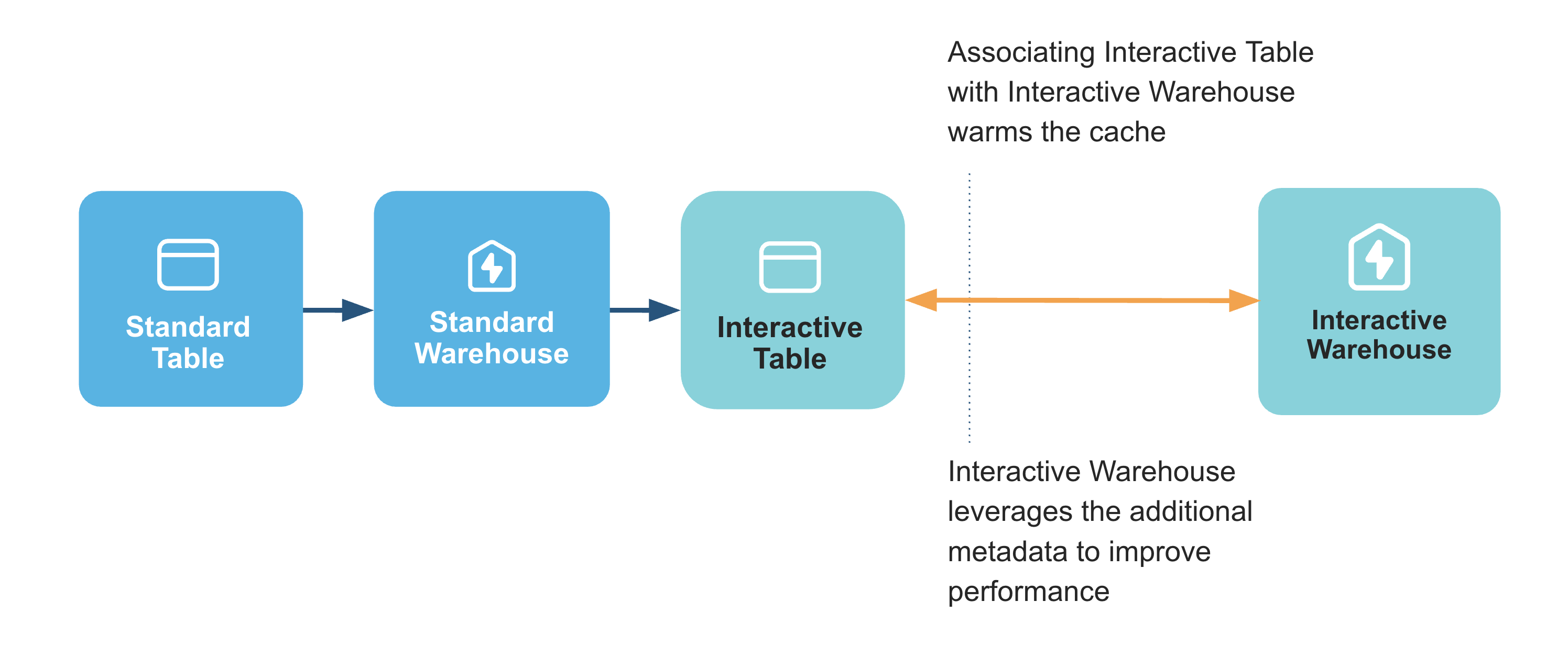
Next, we'll attach our interactive table to the warehouse, which pre-warms the data cache for optimal query performance:
query = """
USE DATABASE MY_DEMO_DB;
"""
execute_and_print(query)

query = """
ALTER WAREHOUSE interactive_demo_b ADD TABLES(BENCHMARK_INTERACTIVE.CUSTOMERS);
"""
execute_and_print(query)
Running the above statement should yield the following:
--------------------------------
Statement executed successfully.
--------------------------------
...
Run queries with interactive warehouse

Now, we'll run our first performance test on the interactive setup by executing a page-view query, timing its execution, and then plotting the results.
We'll start by activating the interactive warehouse and disabling the result cache:
print("Use a standard warehouse for creating the interactive table's data")
cursor.execute("USE WAREHOUSE interactive_demo_b")
cursor.execute('USE DATABASE MY_DEMO_DB;')
cursor.execute('ALTER SESSION SET USE_CACHED_RESULT = FALSE;')

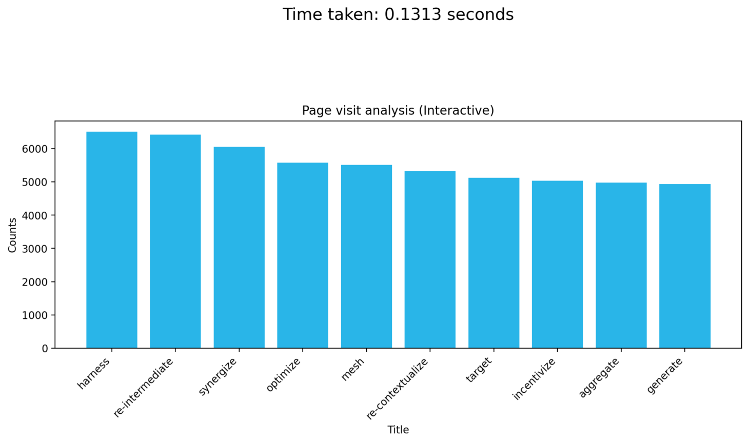
Next, we'll run a query to find the top 10 most viewed pages for July 2013, measures how long it takes, and then plots the results and execution time:
query = """
SELECT Title, COUNT(*) AS PageViews
FROM BENCHMARK_INTERACTIVE.CUSTOMERS
WHERE CounterID = 62
  AND EventDate >= '2013-07-01'
  AND EventDate <= '2013-07-31'
  AND DontCountHits = 0
  AND IsRefresh = 0
  AND Title <> ''
  AND REGEXP_LIKE(Title, '^[\\x00-\\x7F]+$')
  AND LENGTH(Title) < 20
GROUP BY Title
ORDER BY PageViews DESC
LIMIT 10;
"""

start_time = time.time()
result = cursor.execute(query).fetchall()
end_time = time.time()
time_taken = end_time - start_time

plot_data(result, "Page visit analysis (Interactive)", time_taken)
This gives the following plot:
Compare to a standard warehouse

To establish a performance baseline, we'll run an identical page-view query on a standard warehouse to measure and plot its results for comparison.
We'll start by preparing the session for a performance benchmark by selecting a standard WH warehouse, disabling the result cache, and setting the active database:
print("Use a standard warehouse for creating the interactive table's data")
cursor.execute("USE WAREHOUSE WH")
cursor.execute('ALTER SESSION SET USE_CACHED_RESULT = FALSE;')
cursor.execute('USE DATABASE MY_DEMO_DB;')

Here, we'll run a top 10 page views analysis by executing the query, measuring its performance, and immediately plotting the results and execution time:
query = """
SELECT Title, COUNT(*) AS PageViews
FROM BENCHMARK_FDN.HITS2_CSV
WHERE CounterID = 62
  AND EventDate >= '2013-07-01'
  AND EventDate <= '2013-07-31'
  AND DontCountHits = 0
  AND IsRefresh = 0
  AND Title <> ''
  AND REGEXP_LIKE(Title, '^[\\x00-\\x7F]+$')
  AND LENGTH(Title) < 20
GROUP BY Title
ORDER BY PageViews DESC
LIMIT 10;
"""

start_time = time.time()
result = cursor.execute(query).fetchall()
end_time = time.time()
time_taken = end_time - start_time

plot_data(result, "Page visit analysis (Standard)", time_taken, '#5B5B5B')

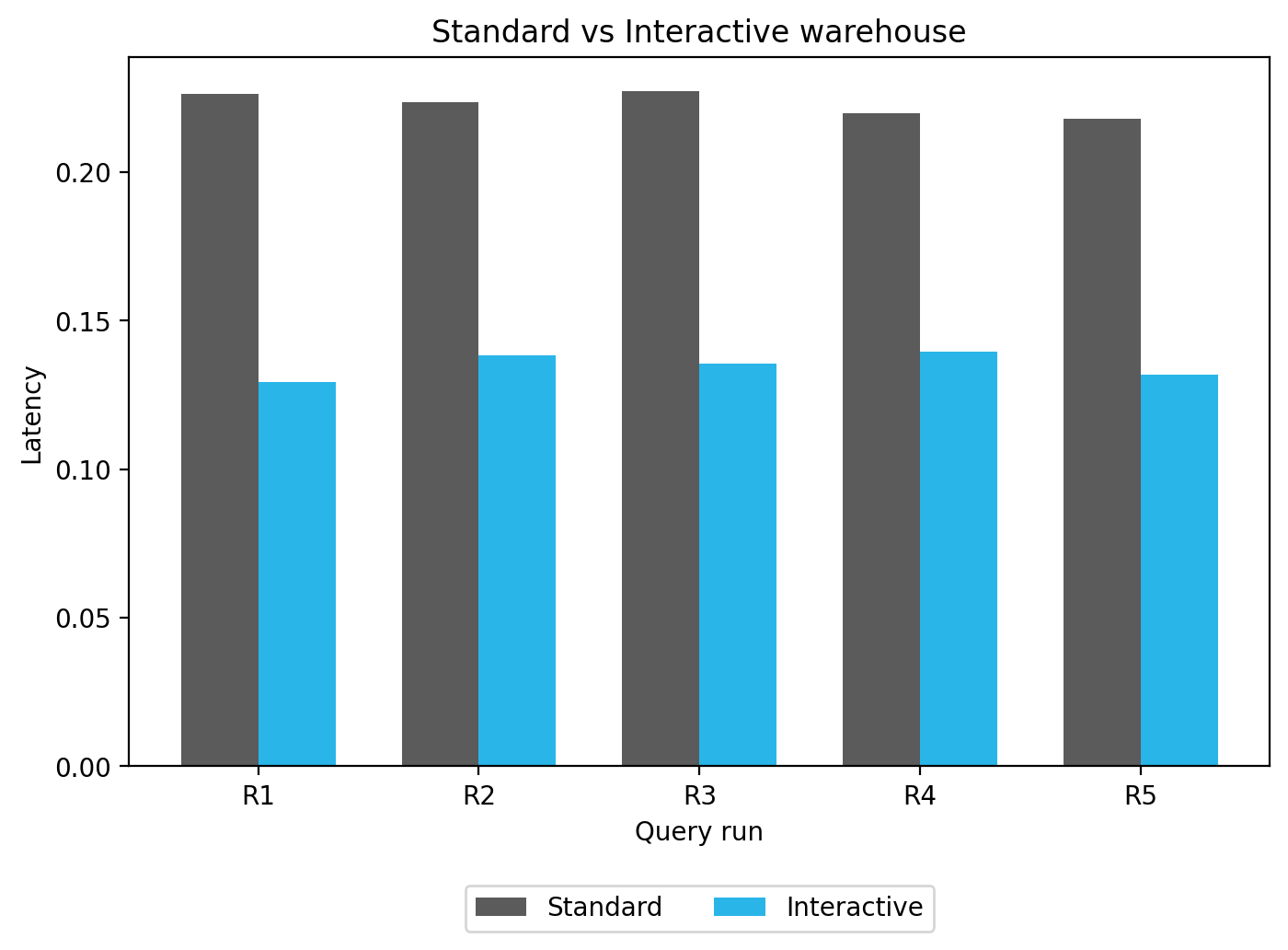
Run some queries concurrently
To directly compare performance, we'll benchmark both the interactive and standard warehouses over several runs and then plot their latencies side-by-side in a grouped bar chart:
runs = 5

counts_iw = run_and_measure(runs,"iw")
print(counts_iw)

counts_std = run_and_measure(runs,"std")
print(counts_std)

titles = [f"R{i}" for i in range(1, len(counts_iw)+1)]

x = np.arange(len(titles))  # the label locations
width = 0.35  # bar width

fig, ax = plt.subplots(figsize=(8, 5))
ax.bar(x - width/2, counts_std, width, label="Standard", color="#5B5B5B")
ax.bar(x + width/2, counts_iw, width, label="Interactive", color="#29B5E8")

ax.set_ylabel("Latency")
ax.set_xlabel("Query run")
ax.set_title("Standard vs Interactive warehouse")
ax.set_xticks(x)
ax.set_xticklabels(titles)
ax.legend(
    loc='upper center',
    bbox_to_anchor=(0.5, -0.15),
    ncol=2
)
plt.show()
Conclusion And Resources
In this guide, we explored how to address the challenge of low-latency, near real-time analytics using Snowflake's interactive warehouses and tables. We walked through the complete setup process, from creating the necessary database objects and loading data to configuring and attaching an interactive table to an interactive warehouse. The subsequent performance benchmark clearly demonstrated the substantial latency improvements these specialized features provide over standard configurations, especially under concurrent query loads. This confirms their value as a powerful solution for demanding use cases like live dashboards and high-throughput data APIs, where sub-second performance is critical.
What You Learned
- Interactive warehouses and tables work together as a specialized pair to deliver low-latency analytics for use cases like live dashboards and APIs.
- How to create, configure, and attach interactive warehouses and tables using SQL to prepare a high-performance analytics environment.
- How to benchmark and visually demonstrate the performance gains of interactive setups over standard ones using Python, proving their effectiveness for high-concurrency workloads.
Related Resources
Data and Notebook:
Documentation:
This content is provided as is, and is not maintained on an ongoing basis. It may be out of date with current Snowflake instances